
Credit risk and repayment capacity
Separate willingness, ability, exposure, and loss severity.
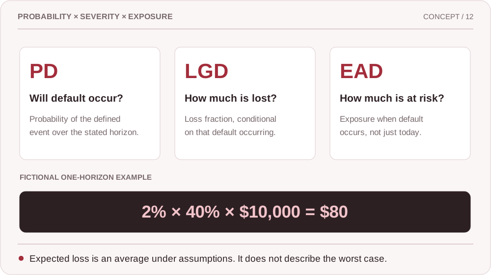
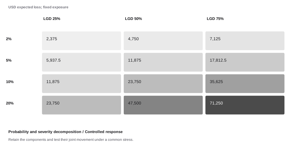
Probability × severity × exposure
Enlarge to read every label and explore the connections
Expected loss combines three different estimates. Define the default event and time horizon before you multiply them.
Define default and the forecast horizon first.
Read each factor as a different question.
Treat the result as an estimate, not a loss limit.
A borrower can have a real identity, an honest intention, and no money when the payment is due. Credit risk is the gap between a promise and the ability to keep it. Fraud controls help, but they do not replace repayment analysis.
Separate default probability and loss severity
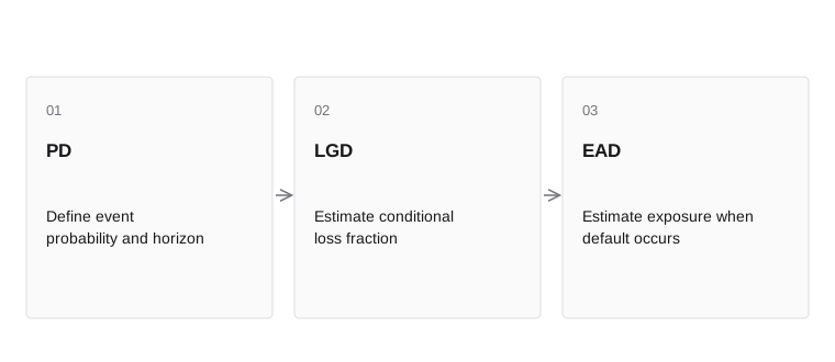
- PDDefine event probability and horizon
- LGDEstimate conditional loss fraction
- EADEstimate exposure when default occurs
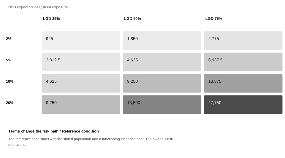
Probability of default estimates the chance that a defined default event occurs over a defined horizon. Loss given default estimates the loss fraction if default occurs. Exposure at default estimates the amount at risk then. A simple expected-loss model multiplies these quantities.
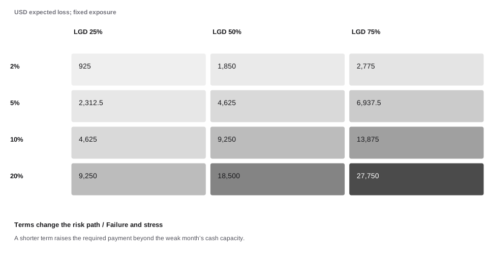
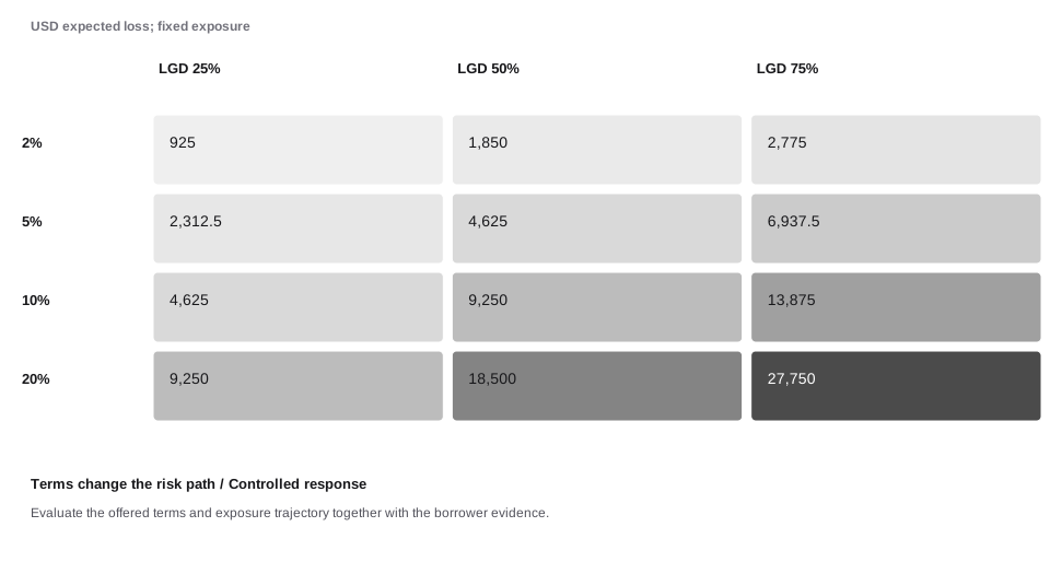
State the default definition and horizon before comparing estimates. A missed payment, a thirty-day delinquency, and a charged-off account are different events. In a teaching example, 4 percent probability, 50 percent loss severity, and $10,000 exposure imply $200 expected loss. This simplified result excludes timing, uncertainty, and other accounting or capital requirements.
Probability of default, loss given default, and exposure at default describe different uncertainties. A borrower can have a modest chance of default but create a large loss if there is little usable recovery. Another can default more often while producing lower losses because exposure is smaller or recoveries are stronger. The simplified product PD × LGD × EAD is an expected value over stated assumptions, not a complete accounting standard or a description of the worst case.
These quantities can also move together under stress. A downturn may increase defaults at the same time that collateral loses value and customers draw unused commitments. Treating each input as an independent fixed average can understate the combined event. A stress case should explain how the shared cause affects all relevant components.
Inside the mechanism. Expected loss in a simplified model is exposure at default multiplied by probability of default and loss given default for a stated horizon. The components are not interchangeable. Better collateral may reduce severity without reducing the borrower’s chance of default. A one-year probability cannot be applied as a monthly probability. This teaching calculation is not an accounting allowance method; real estimation needs definitions, dependence, timing, and applicable accounting treatment.
A concrete example. Two borrowers can have the same expected loss for different reasons. One defaults more often; the other produces a larger loss when default occurs. The case has $475,000 of exposure. Its stated one-year PD and LGD imply $10,307.50 of expected loss, while the cover analysis leaves $349,000.00 of stress exposure. Monthly cash coverage is 1.50×. These are separate measures: one describes an average under probability assumptions, one describes available cover, and one describes a period’s funding capacity.
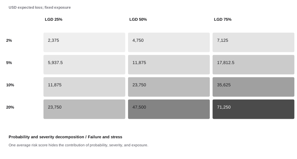
When the assumption fails. One average risk score hides the contribution of probability, severity, and exposure. Retain the components and test their joint movement under a common stress. The following worked sequence shows the reference condition, a stress condition, and a response condition with explicit synthetic data. These are comparative assumptions, not measured causal effects.
Two borrowers can have the same expected loss for different reasons. One defaults more often; the other produces a larger loss when default occurs.
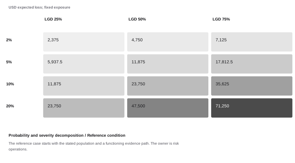
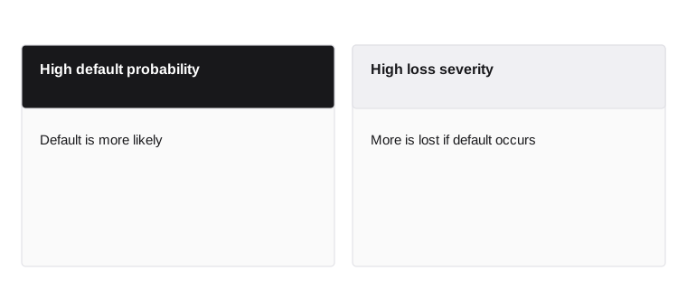
- High default probability
- Default is more likely
- High loss severity
- More is lost if default occurs
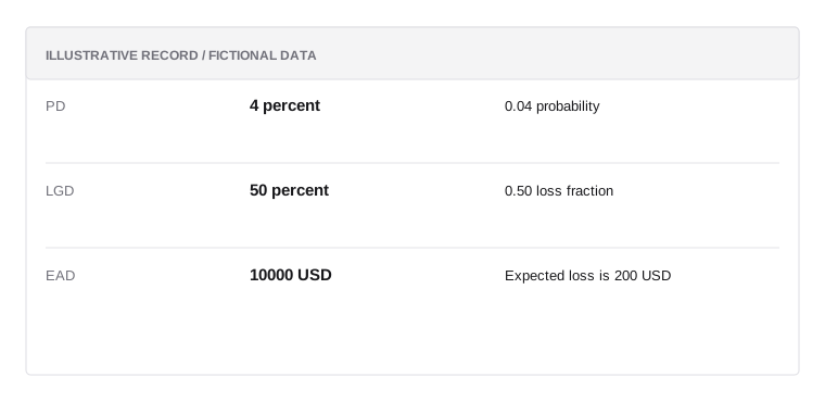
Expected-loss example
Illustrative data; not a real customer record or a prescribed policy.
- PD4 percent
0.04 probability
- LGD50 percent
0.50 loss fraction
- EAD10000 USD
Expected loss is 200 USD
Each changes expected loss differently
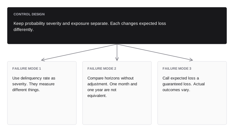
Keep probability severity and exposure separate. Each changes expected loss differently.
- Failure mode 1avoid
- Use delinquency rate as severity. They measure different things.
- Failure mode 2avoid
- Compare horizons without adjustment. One month and one year are not equivalent.
- Failure mode 3avoid
- Call expected loss a guaranteed loss. Actual outcomes vary.
Assess cash available for repayment
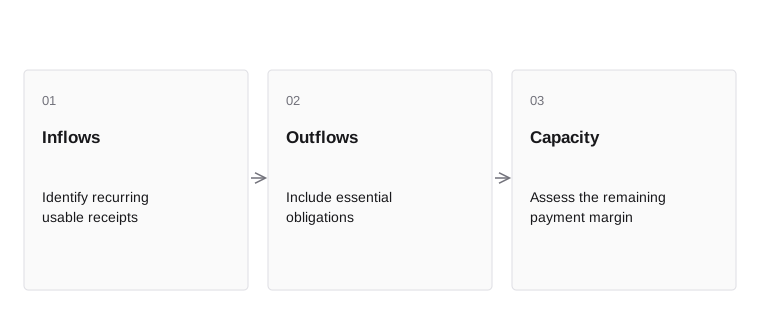
- InflowsIdentify recurring usable receipts
- OutflowsInclude essential obligations
- CapacityAssess the remaining payment margin
Revenue is not cash available for debt service. Operating costs, taxes, existing obligations, working-capital needs, and timing all affect repayment capacity. Use a consistent period and distinguish recurring inflows from one-time transfers.
A business with $100,000 monthly receipts and $85,000 essential outflows has $15,000 before the proposed debt payment under these simplified assumptions. A $12,000 payment leaves a narrow $3,000 margin. Test sensitivity to lower sales or delayed receipts. The decision should reflect the actual product terms and verified evidence, not only a favorable average month.
Inside the mechanism. Repayment capacity depends on cash available during the repayment period after necessary operating demands. State which receipts and costs enter the calculation and whether they are recurring. A coverage ratio with an undefined numerator is difficult to interpret. Test the weak period rather than relying only on annual averages. A business can show positive annual cash generation while failing a large installment before seasonal receipts arrive.
A concrete example. Revenue and accounting profit do not automatically equal cash available for a scheduled payment. The useful measure follows the cash after relevant operating needs. The case has $225,000 of exposure. Its stated one-year PD and LGD imply $6,187.50 of expected loss, while the cover analysis leaves $174,000.00 of stress exposure. Monthly cash coverage is 1.20×. These are separate measures: one describes an average under probability assumptions, one describes available cover, and one describes a period’s funding capacity.
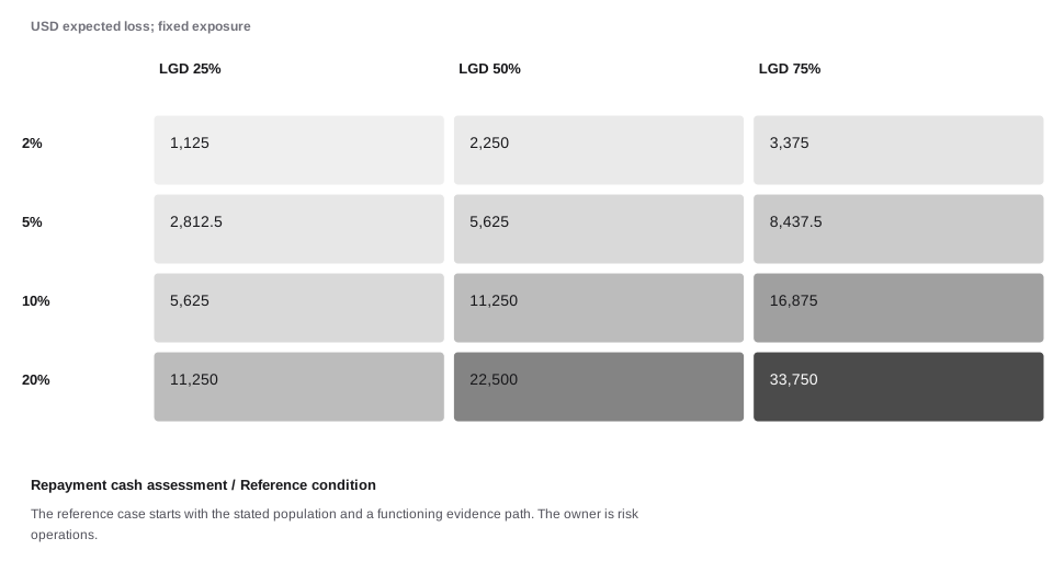
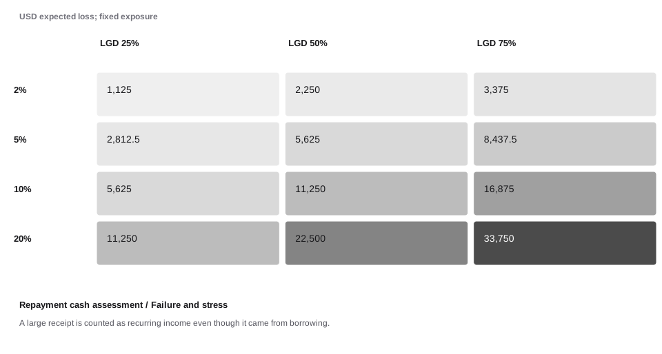
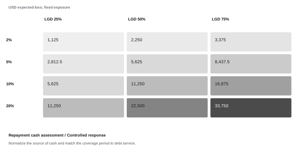
When the assumption fails. A large receipt is counted as recurring income even though it came from borrowing. Normalize the source of cash and match the coverage period to debt service. The following worked sequence shows the reference condition, a stress condition, and a response condition with explicit synthetic data. These are comparative assumptions, not measured causal effects.
Revenue and accounting profit do not automatically equal cash available for a scheduled payment. The useful measure follows the cash after relevant operating needs.
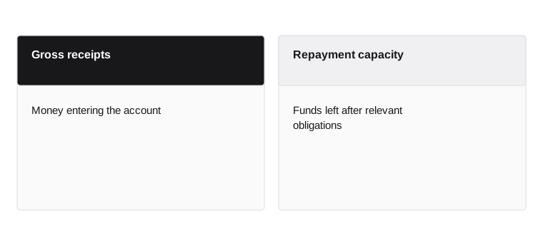
- Gross receipts
- Money entering the account
- Repayment capacity
- Funds left after relevant obligations
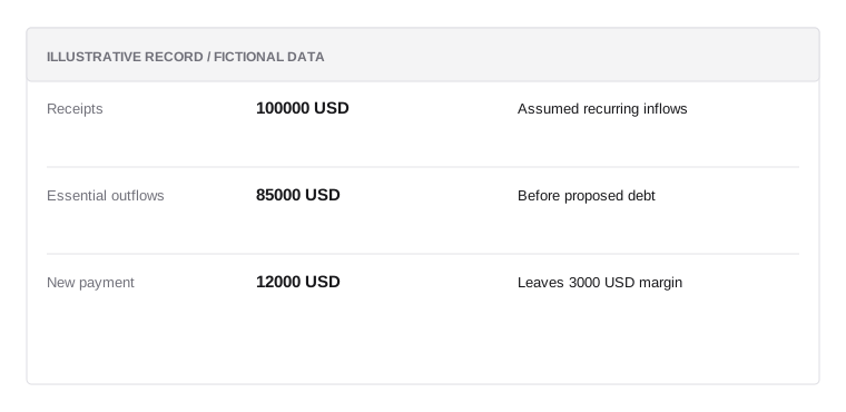
Monthly capacity example
Illustrative data; not a real customer record or a prescribed policy.
- Receipts100000 USD
Assumed recurring inflows
- Essential outflows85000 USD
Before proposed debt
- New payment12000 USD
Leaves 3000 USD margin
Receipts alone overstate available capacity
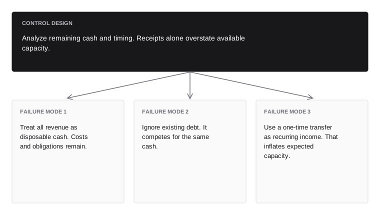
Analyze remaining cash and timing. Receipts alone overstate available capacity.
- Failure mode 1avoid
- Treat all revenue as disposable cash. Costs and obligations remain.
- Failure mode 2avoid
- Ignore existing debt. It competes for the same cash.
- Failure mode 3avoid
- Use a one-time transfer as recurring income. That inflates expected capacity.
Distinguish fraud and credit evidence
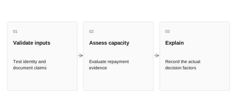
- Validate inputsTest identity and document claims
- Assess capacityEvaluate repayment evidence
- ExplainRecord the actual decision factors
False income documents concern deception. A genuine income decline concerns capacity. Both can lead to nonpayment but require different controls and customer responses. Keep the reason for a credit decision specific to the evidence and applicable requirements.
Use identity and document checks to establish trustworthy inputs, then assess repayment with those inputs. A high identity confidence score does not mean low default probability. Conversely, a borrower with limited credit history is not necessarily using a false identity. Avoid a single opaque risk label that mixes fraud, affordability, and legal eligibility.
Inside the mechanism. Fraud evidence concerns the reliability or authenticity of the claim and conduct; credit evidence concerns the ability and willingness to meet an obligation under the relevant facts. They can interact without being the same label. A genuine business with falling revenue may be a credit problem. Fabricated bank statements create a different evidentiary concern. Preserve the distinction so the response, notice, investigation, and future model target remain appropriate.
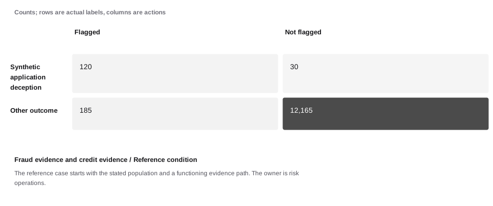
A concrete example. A borrower can intend to repay and still default; a fraudulent application can also make early payments. The target definition determines what the model is learning. The rule flags 305 of 12,500 credit applications. Of those flags, 120 meet the synthetic target, giving 39.34% precision. It misses 30 target events. Under the stated cost assumptions, residual loss and operating friction total $108,415. The important result is the connection between the population, action, capacity, and outcome—not one isolated score.
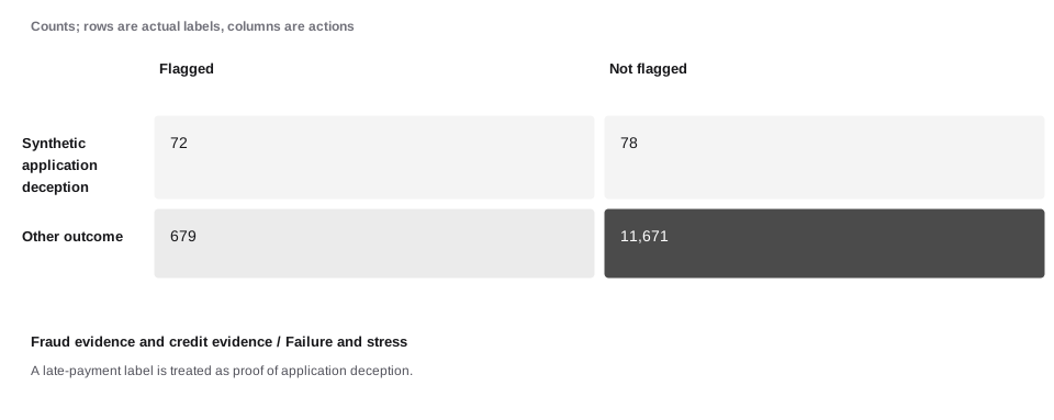
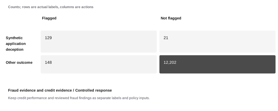
When the assumption fails. A late-payment label is treated as proof of application deception. Keep credit performance and reviewed fraud findings as separate labels and policy inputs. The following worked sequence shows the reference condition, a stress condition, and a response condition with explicit synthetic data. These are comparative assumptions, not measured causal effects.
A borrower can intend to repay and still default; a fraudulent application can also make early payments. The target definition determines what the model is learning.
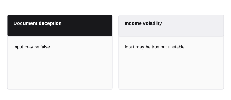
- Document deception
- Input may be false
- Income volatility
- Input may be true but unstable
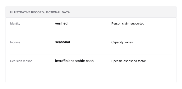
Borrower evidence
Illustrative data; not a real customer record or a prescribed policy.
- Identityverified
Person claim supported
- Incomeseasonal
Capacity varies
- Decision reasoninsufficient stable cash
Specific assessed factor
They address different uncertainties
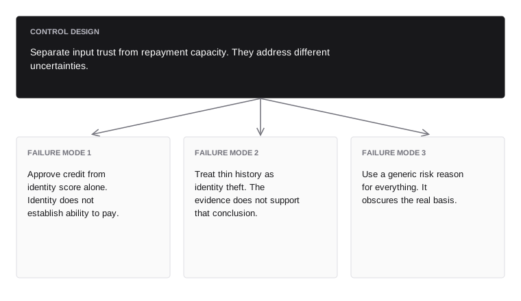
Separate input trust from repayment capacity. They address different uncertainties.
- Failure mode 1avoid
- Approve credit from identity score alone. Identity does not establish ability to pay.
- Failure mode 2avoid
- Treat thin history as identity theft. The evidence does not support that conclusion.
- Failure mode 3avoid
- Use a generic risk reason for everything. It obscures the real basis.
Model terms and behavior together
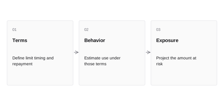
- TermsDefine limit timing and repayment
- BehaviorEstimate use under those terms
- ExposureProject the amount at risk
A limit, payment schedule, maturity, and pricing structure affect exposure and customer behavior. A larger revolving limit can increase future drawn exposure even if today’s balance is small. A short repayment cycle can strain a seasonal business.
Evaluate the proposed terms as part of the decision, not as an afterthought. Use scenarios for utilization, repayment, and stress. Distinguish an approved limit from a funded balance and from projected exposure at default. The three may differ substantially. Reassess terms through an approved process when the underlying evidence changes.
Loan terms change borrower behavior and the platform’s exposure. A shorter repayment period may reduce time at risk while increasing the payment burden. A larger limit may improve the customer’s flexibility while increasing the amount outstanding when conditions worsen. Model and policy reviews should therefore consider the offered terms, not just whether an applicant receives a binary approval. A decision record is stronger when it explains both eligibility and the particular amount, duration, or conditions offered.
Inside the mechanism. Terms change exposure and behavior. A shorter repayment interval, smaller advance, or slower payout can alter both the cash path and the customer’s operating capacity. Model the proposed terms with the business cycle rather than treating the score as independent of the offer. A control that removes working capital can also weaken fulfillment. Record the assumptions behind the offer and monitor whether the actual behavior remains within them.
A concrete example. Amount, payment schedule, and duration affect utilization and repayment pressure. Eligibility alone does not describe the offer that the customer actually receives. The case has $185,000 of exposure. Its stated one-year PD and LGD imply $6,613.75 of expected loss, while the cover analysis leaves $126,000.00 of stress exposure. Monthly cash coverage is 0.97×. These are separate measures: one describes an average under probability assumptions, one describes available cover, and one describes a period’s funding capacity.
When the assumption fails. A shorter term raises the required payment beyond the weak month’s cash capacity. Evaluate the offered terms and exposure trajectory together with the borrower evidence. The following worked sequence shows the reference condition, a stress condition, and a response condition with explicit synthetic data. These are comparative assumptions, not measured causal effects.
Amount, payment schedule, and duration affect utilization and repayment pressure. Eligibility alone does not describe the offer that the customer actually receives.
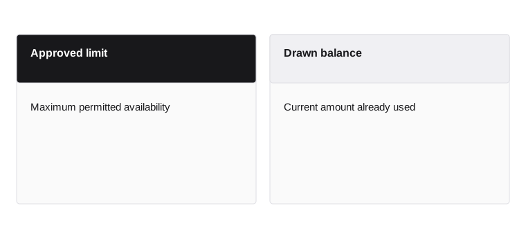
- Approved limit
- Maximum permitted availability
- Drawn balance
- Current amount already used
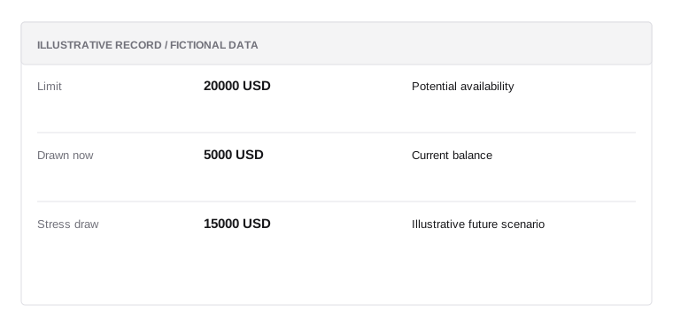
Revolving-line example
Illustrative data; not a real customer record or a prescribed policy.
- Limit20000 USD
Potential availability
- Drawn now5000 USD
Current balance
- Stress draw15000 USD
Illustrative future scenario
Current balance may understate later exposure
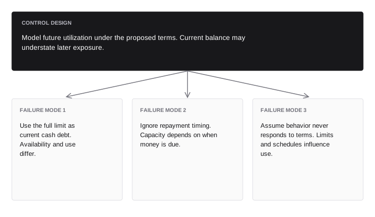
Model future utilization under the proposed terms. Current balance may understate later exposure.
- Failure mode 1avoid
- Use the full limit as current cash debt. Availability and use differ.
- Failure mode 2avoid
- Ignore repayment timing. Capacity depends on when money is due.
- Failure mode 3avoid
- Assume behavior never responds to terms. Limits and schedules influence use.
Preserve a reasoned decision record
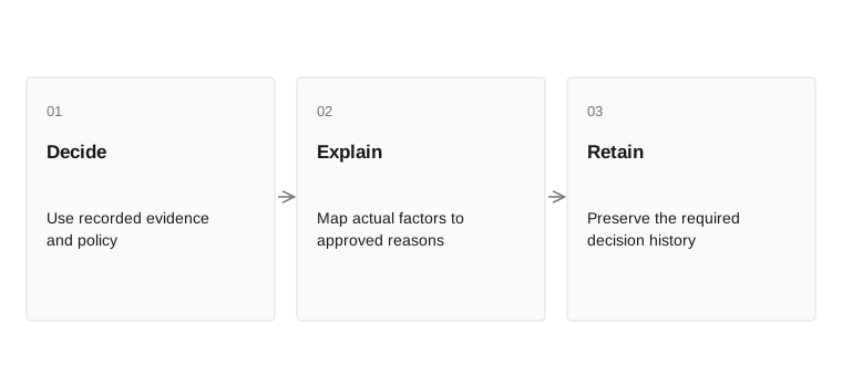
- DecideUse recorded evidence and policy
- ExplainMap actual factors to approved reasons
- RetainPreserve the required decision history
Record the application state, evidence, model and policy versions, decision, and actual reasons. Credit decisions can carry notice and record duties that vary by product and applicant. The implementation must map those duties to the correct lifecycle event.
A technical explanation is not automatically a compliant customer explanation. A model feature may need translation into a specific, accurate reason through an approved process. Keep that translation versioned and test it against actual decisions. Do not invent a convenient reason after the fact because the model cannot explain itself.
Inside the mechanism. A reasoned decision record ties material facts to the actual terms or action. Retain the data used, its date, relevant model and policy versions, principal decision factors, overrides, and approval authority. A later explanation should not reconstruct reasons from a different model. The record also supports review of inconsistent treatment and data errors. Applicable notice requirements need their own tested workflow rather than being assumed satisfied by an internal score log.
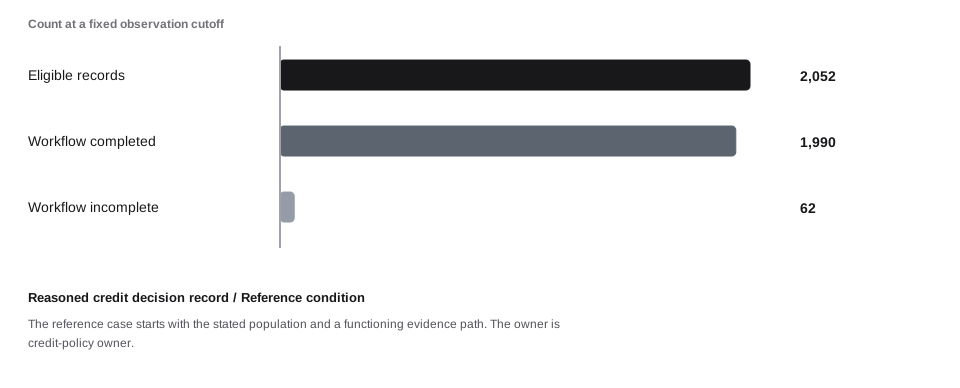
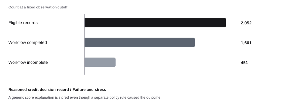
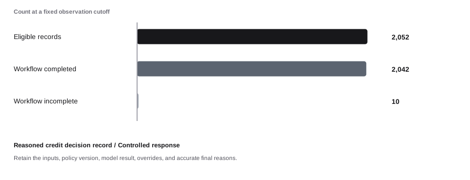
A concrete example. A reviewer must reconstruct why the offered terms or adverse action followed from the facts. The final record needs the actual decision path. The case identifies 2,052 eligible records from a source population of 2,700. The required workflow completes for 1,990, but 30 completed records miss the illustrative internal target. Another 62 remain incomplete. Communication evidence covers 1,970 generated notices. Scope, completion, timeliness, and delivery are four separate properties of the customer outcome.
When the assumption fails. A generic score explanation is stored even though a separate policy rule caused the outcome. Retain the inputs, policy version, model result, overrides, and accurate final reasons. The following worked sequence shows the reference condition, a stress condition, and a response condition with explicit synthetic data. These are comparative assumptions, not measured causal effects.
A reviewer must reconstruct why the offered terms or adverse action followed from the facts. The final record needs the actual decision path.
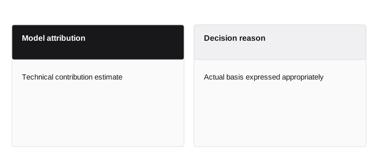
- Model attribution
- Technical contribution estimate
- Decision reason
- Actual basis expressed appropriately
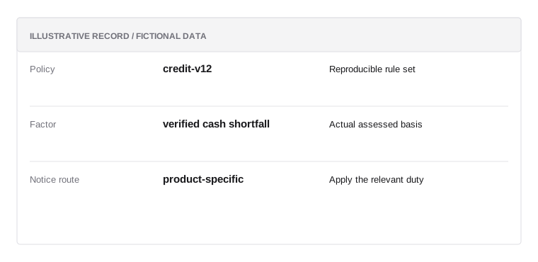
Credit decision record
Illustrative data; not a real customer record or a prescribed policy.
- Policycredit-v12
Reproducible rule set
- Factorverified cash shortfall
Actual assessed basis
- Notice routeproduct-specific
Apply the relevant duty
The explanation must reflect what actually drove it
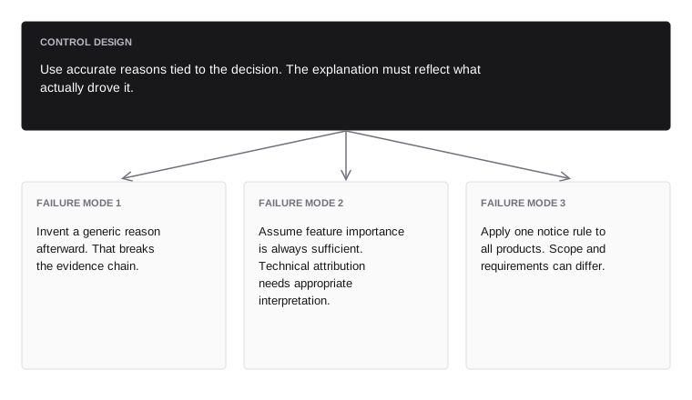
Use accurate reasons tied to the decision. The explanation must reflect what actually drove it.
- Failure mode 1avoid
- Invent a generic reason afterward. That breaks the evidence chain.
- Failure mode 2avoid
- Assume feature importance is always sufficient. Technical attribution needs appropriate interpretation.
- Failure mode 3avoid
- Apply one notice rule to all products. Scope and requirements can differ.
Chapter connections
This chapter builds on Underwrite the merchant business. Continue with Cash-flow analysis and financial evidence to follow the next part of the system. Use the glossary for terminology and risk mathematics for formulas and worked calculations.