
Repayment cash assessment
Assess cash available for repayment
Separate probability, severity, and exposure
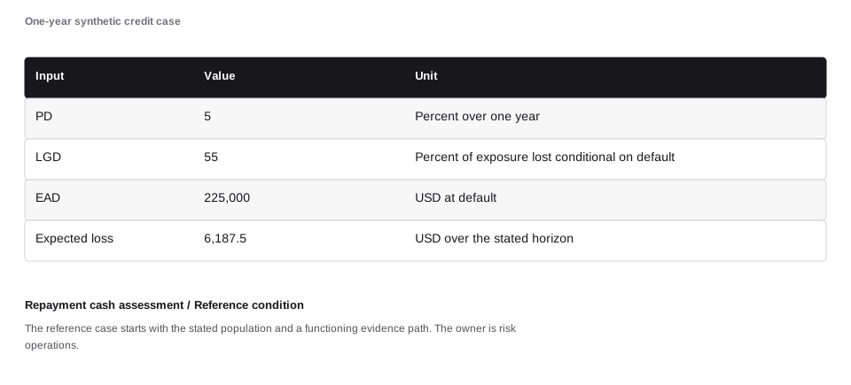
The simplified one-year expected loss is PD × LGD × EAD = $6,187.50. PD is 5.00%, LGD is 55.00%, and EAD is $225,000. This is a teaching expected-value calculation, not an accounting allowance method or a capital standard.
Figure data and text version
| Input | Value | Unit |
|---|---|---|
| PD | 5 | Percent over one year |
| LGD | 55 | Percent of exposure lost conditional on default |
| EAD | 225,000 | USD at default |
| Expected loss | 6,187.5 | USD over the stated horizon |
Revenue and accounting profit do not automatically equal cash available for a scheduled payment. The useful measure follows the cash after relevant operating needs.
The reference case starts with the stated population and a functioning evidence path. The owner is risk operations.
All amounts, rates, capacity limits, and outcomes in this case are synthetic. The three conditions are separate assumptions for comparison. A better result in the response condition is not measured proof that the proposed control causes that improvement. The figures expose the calculation and its limits; a real deployment needs its own evidence.
Read the result
The case has $225,000 of exposure. Its stated one-year PD and LGD imply $6,187.50 of expected loss, while the cover analysis leaves $174,000.00 of stress exposure. Monthly cash coverage is 1.20×. These are separate measures: one describes an average under probability assumptions, one describes available cover, and one describes a period’s funding capacity.
Model inputs and calculated values
Inputs below are the case-specific values. Each figure states the condition-specific assumptions and units used in its calculation. Calculated values are rounded for display.
| Input | Value |
|---|---|
| exposure | 225,000 |
| pd | 0.05 |
| cash | 16,800 |
| debtService | 14,000 |
| collateral | 45,000 |
| Calculated value | Result |
|---|---|
| ead | 225,000 |
| pd | 0.05 |
| lgd | 0.55 |
| expectedLoss | 6,187.5 |
| eligibleCover | 36,000 |
| reserve | 15,000 |
| uncovered | 174,000 |
| cash | 16,800 |
| debt | 14,000 |
| dscr | 1.2 |
Probability and severity move the result together
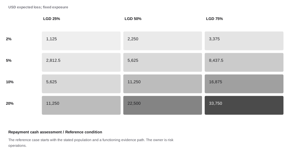
Each cell is the same exposure multiplied by the row default probability and the column loss severity. The grid makes joint stress visible. A downturn can affect both factors; the calculation does not assume that the two causes are independent.
Figure data and text version
| PD | LGD 25% | LGD 50% | LGD 75% |
|---|---|---|---|
| 2% | 1,125 | 2,250 | 3,375 |
| 5% | 2,812.5 | 5,625 | 8,437.5 |
| 10% | 5,625 | 11,250 | 16,875 |
| 20% | 11,250 | 22,500 | 33,750 |
Recorded collateral and eligible cover
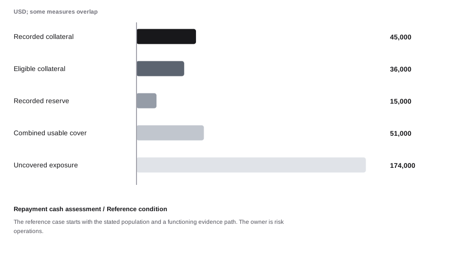
The collateral record is $45,000, but a 20% illustrative haircut leaves $36,000.00 eligible in this scenario. Reserve cover adds $15,000. The resulting uncovered exposure is $174,000.00. Eligibility also needs enforceability and operational access; this arithmetic does not establish either.
Figure data and text version
| Measure | USD |
|---|---|
| Recorded collateral | 45,000 |
| Eligible collateral | 36,000 |
| Recorded reserve | 15,000 |
| Combined usable cover | 51,000 |
| Uncovered exposure | 174,000 |
Cash available for the period’s debt service
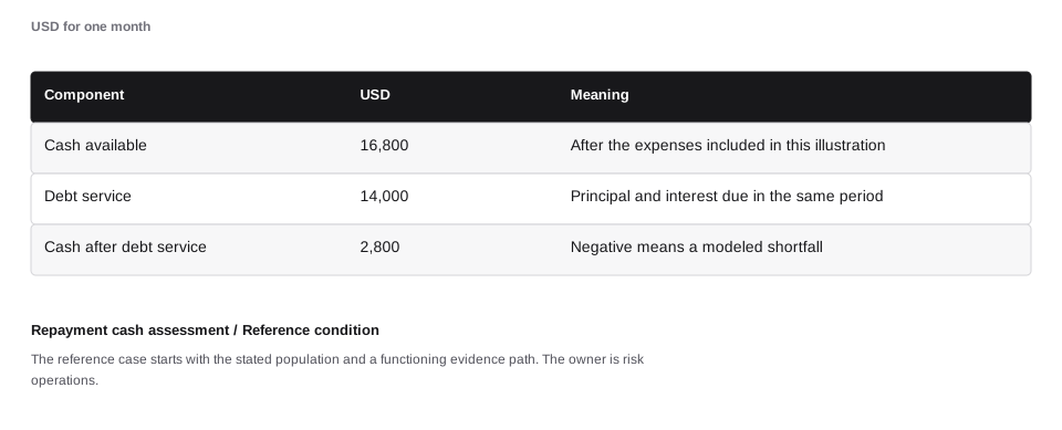
Defined cash available is $16,800.00 against $14,000.00 of debt service, for a 1.20× ratio. The ratio uses one period and one defined cash measure. It does not establish affordability, suitability, or a required underwriting threshold.
Figure data and text version
| Component | USD | Meaning |
|---|---|---|
| Cash available | 16,800 | After the expenses included in this illustration |
| Debt service | 14,000 | Principal and interest due in the same period |
| Cash after debt service | 2,800 | Negative means a modeled shortfall |
A constant-hazard illustration
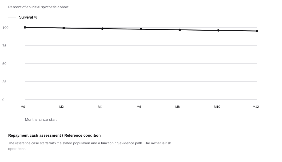
The curve converts the stated one-year PD of 5.00% to a constant monthly hazard using h = 1 − (1 − PD)^(1/12). Survival after 12 months is therefore 1 − PD. Constant hazard is an assumption; seasonality and changing exposure are omitted. Horizontal positions are the labeled observations or scenarios; equal spacing does not imply equal numerical increments.
Figure data and text version
| Months since start | Survival % |
|---|---|
| M0 | 100 |
| M2 | 99.15 |
| M4 | 98.3 |
| M6 | 97.47 |
| M8 | 96.64 |
| M10 | 95.82 |
| M12 | 95 |
Cumulative expected loss at comparable age
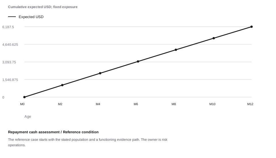
This curve multiplies cumulative modeled default probability by a fixed EAD and LGD. It is useful for separating observation age from the chosen assumptions. It omits amortization, recoveries over time, prepayment, and changing utilization. Horizontal positions are the labeled observations or scenarios; equal spacing does not imply equal numerical increments.
Figure data and text version
| Age | Expected USD |
|---|---|
| M0 | 0 |
| M2 | 1,053.42 |
| M4 | 2,097.86 |
| M6 | 3,133.42 |
| M8 | 4,160.16 |
| M10 | 5,178.16 |
| M12 | 6,187.5 |
Expected loss sensitivity to PD
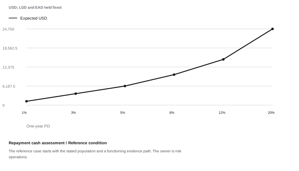
Exposure stays at $225,000 and LGD stays at 55.00% while PD changes. The linear relationship follows the simplified expected-loss formula. It is not evidence that real-world losses respond linearly to economic stress. Horizontal positions are the labeled observations or scenarios; equal spacing does not imply equal numerical increments.
Figure data and text version
| One-year PD | Expected USD |
|---|---|
| 1% | 1,237.5 |
| 3% | 3,712.5 |
| 5% | 6,187.5 |
| 8% | 9,900 |
| 12% | 14,850 |
| 20% | 24,750 |
A shared dependency can dominate exposure
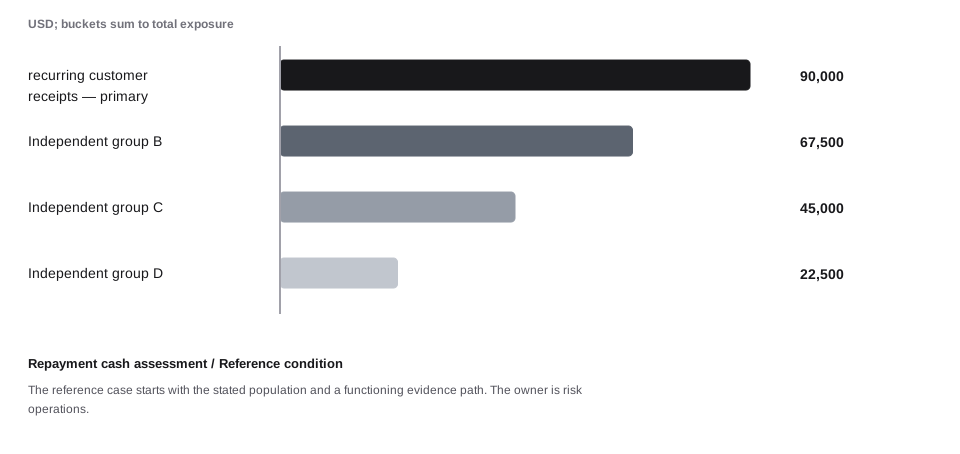
The four amounts are disjoint portions of this case’s exposure. The largest bucket represents one shared supplier, funding source, or other specified dependency. Counting customers alone would not reveal this common loss driver.
Figure data and text version
| Dependency bucket | Exposure USD |
|---|---|
| recurring customer receipts — primary | 90,000 |
| Independent group B | 67,500 |
| Independent group C | 45,000 |
| Independent group D | 22,500 |
A weak month can disappear inside an average
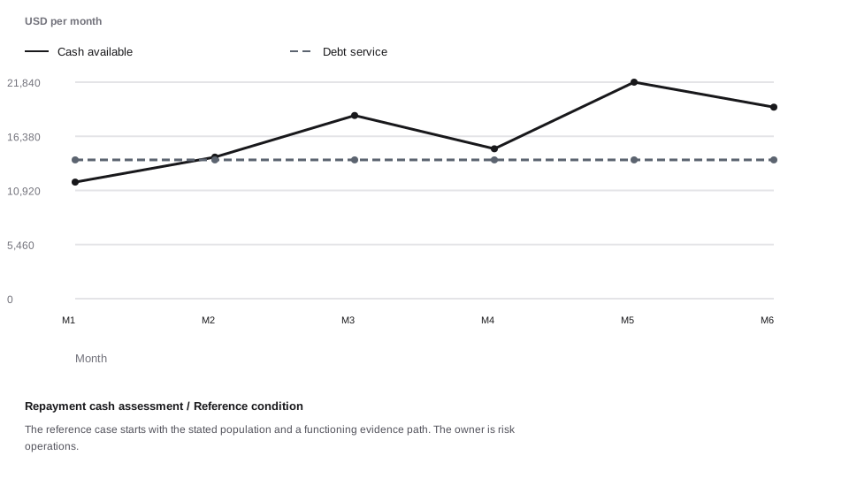
The six-month path applies explicit seasonal factors to the defined monthly cash amount and compares it with fixed debt service. These are constructed cash assumptions, not a forecast. A negative month needs a funding or terms response even when the average ratio looks comfortable. Horizontal positions are the labeled observations or scenarios; equal spacing does not imply equal numerical increments.
Figure data and text version
| Month | Cash available | Debt service |
|---|---|---|
| M1 | 11,760 | 14,000 |
| M2 | 14,280 | 14,000 |
| M3 | 18,480 | 14,000 |
| M4 | 15,120 | 14,000 |
| M5 | 21,840 | 14,000 |
| M6 | 19,320 | 14,000 |
Terms belong in the decision record
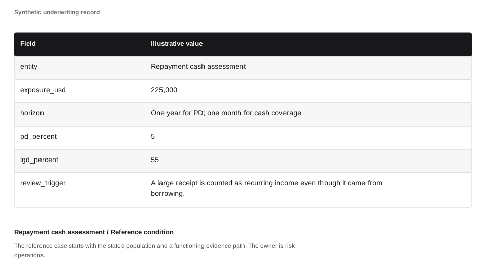
This record concerns assess cash available for repayment. A binary approval omits the amount, observation horizon, cover assumptions, and review trigger. Retaining those terms makes the decision reproducible and identifies when changed facts require another assessment.
Figure data and text version
| Field | Illustrative value |
|---|---|
| entity | Repayment cash assessment |
| exposure_usd | 225,000 |
| horizon | One year for PD; one month for cash coverage |
| pd_percent | 5 |
| lgd_percent | 55 |
| review_trigger | A large receipt is counted as recurring income even though it came from borrowing. |
One cause can affect several loss components
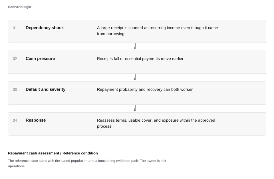
The stress path connects recurring customer receipts to repayment cash, default probability, recovery, and funding needs. Arrows state the scenario’s assumed causal chain. They are hypotheses to test with evidence, not proof that every affected customer will default.
Figure data and text version
| Stage | Mechanism |
|---|---|
| Dependency shock | A large receipt is counted as recurring income even though it came from borrowing. |
| Cash pressure | Receipts fall or essential payments move earlier |
| Default and severity | Repayment probability and recovery can both worsen |
| Response | Reassess terms, usable cover, and exposure within the approved process |
Expected loss, uncovered exposure, and cash gap
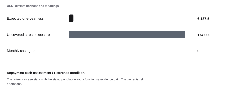
Expected loss ($6,187.50), uncovered exposure ($174,000.00), and monthly cash gap ($0.00) answer different questions. The bars are deliberately separated measures and must not be added. A low expected value can coexist with a large stress exposure.
Figure data and text version
| Measure | USD |
|---|---|
| Expected one-year loss | 6,187.5 |
| Uncovered stress exposure | 174,000 |
| Monthly cash gap | 0 |
Connect the result to the system
Normalize the source of cash and match the coverage period to debt service.
Check the population, evidence, permitted action, and actual effect together. A balanced calculation can still use the wrong population; a successful response can still leave an unknown financial outcome. The case’s numerical result applies only to its stated assumptions.
Sources and further reading
The chapter sources support the concepts and scope. They do not prescribe the synthetic model rates.