
Risk models, calibration, and delayed outcomes
Evaluate predictions against the decision they will support.
A probability must agree with outcomes
Enlarge to read every label and explore the connections
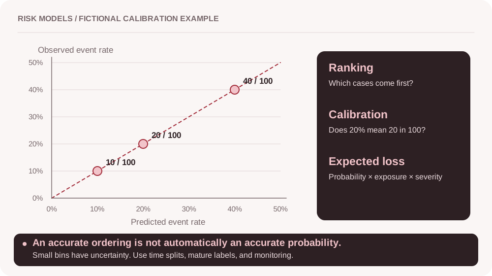
A model can rank cases well while its probabilities are wrong. Check calibration on a defined, mature population before using scores in loss calculations.
Define the target, population, and label maturity.
Compare predicted and observed frequencies.
Separate ranking, calibration, and financial loss.
A model reports 99 percent accuracy. Fraud occurs in only 1 percent of the population. A model that predicts no fraud at all can claim the same number. The interesting result is hidden in the errors.
Choose a target that matches the action
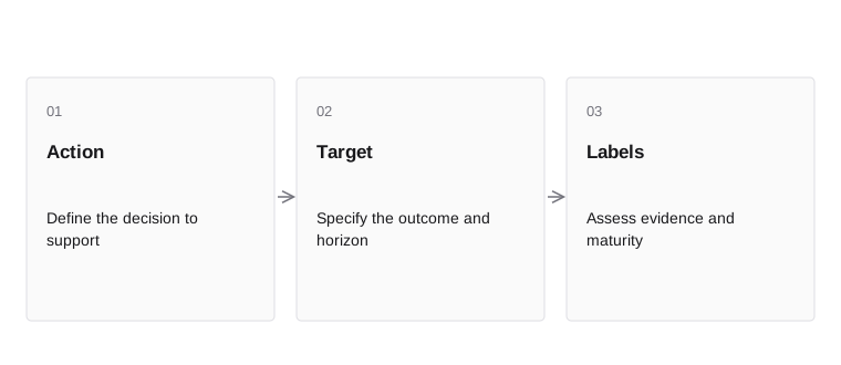
- ActionDefine the decision to support
- TargetSpecify the outcome and horizon
- LabelsAssess evidence and maturity
A model target defines what the system learns to predict. Confirmed unauthorized use, a dispute, a default, and a suspicious-activity disposition are different labels. Choose the target from the intended decision and available evidence.
Specify the prediction horizon, population, exclusions, and label maturity. A payment-fraud model should not silently use merchant service disputes as equivalent fraud labels. A credit model should distinguish a technical payment failure from inability to repay. Write a target contract before selecting the algorithm. Otherwise, a sophisticated model can optimize the wrong outcome very efficiently.
Inside the mechanism. Write the target as an observable outcome with a horizon, unit, amount treatment, exclusions, and maturity rule. A dispute occurrence, confirmed unauthorized payment, and final loss are different targets. Match the intervention to the mechanism the target represents. If the action cannot affect the outcome, a predictive model may still be useful for planning but does not establish preventable loss.
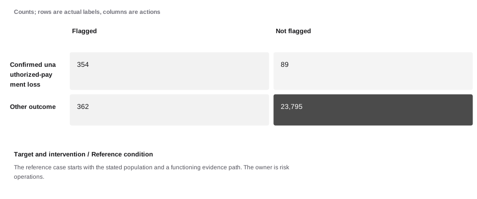
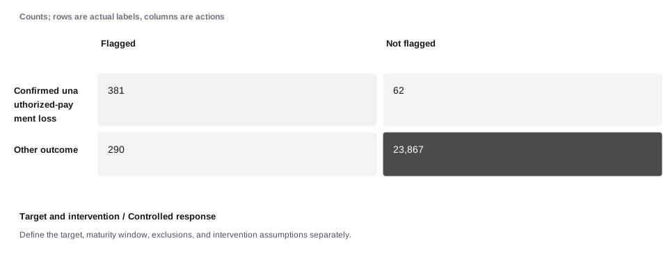
A concrete example. A model trained to predict disputes does not automatically estimate unauthorized fraud or preventable loss. The label should match the outcome and action being evaluated. The rule flags 716 of 24,600 mature transactions. Of those flags, 354 meet the synthetic target, giving 49.44% precision. It misses 89 target events. Under the stated cost assumptions, residual loss and operating friction total $17,579. The important result is the connection between the population, action, capacity, and outcome—not one isolated score.
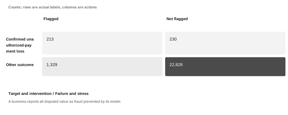
When the assumption fails. A business reports all disputed value as fraud prevented by its model. Define the target, maturity window, exclusions, and intervention assumptions separately. The following worked sequence shows the reference condition, a stress condition, and a response condition with explicit synthetic data. These are comparative assumptions, not measured causal effects.
A model trained to predict disputes does not automatically estimate unauthorized fraud or preventable loss. The label should match the outcome and action being evaluated.
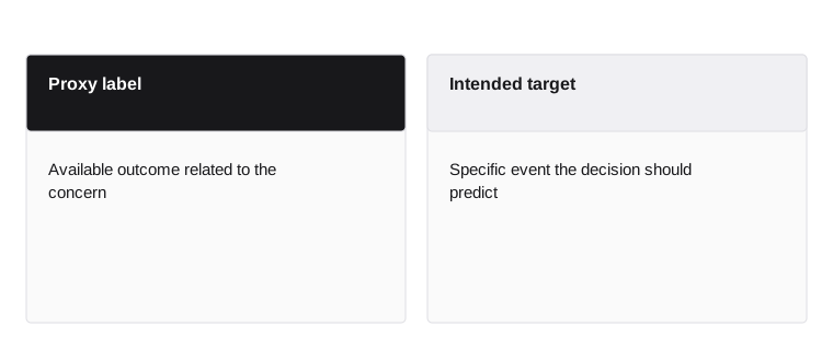
- Proxy label
- Available outcome related to the concern
- Intended target
- Specific event the decision should predict
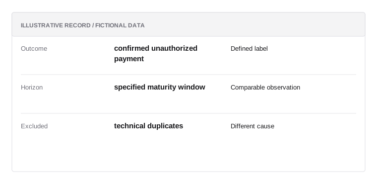
Target contract
Illustrative data; not a real customer record or a prescribed policy.
- Outcomeconfirmed unauthorized payment
Defined label
- Horizonspecified maturity window
Comparable observation
- Excludedtechnical duplicates
Different cause
Different bad outcomes need different controls
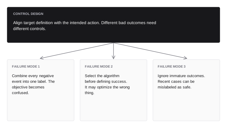
Align target definition with the intended action. Different bad outcomes need different controls.
- Failure mode 1avoid
- Combine every negative event into one label. The objective becomes confused.
- Failure mode 2avoid
- Select the algorithm before defining success. It may optimize the wrong thing.
- Failure mode 3avoid
- Ignore immature outcomes. Recent cases can be mislabeled as safe.
Read the confusion matrix
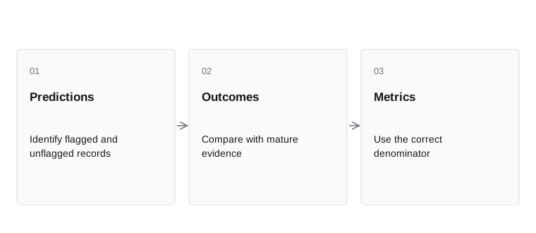
- PredictionsIdentify flagged and unflagged records
- OutcomesCompare with mature evidence
- MetricsUse the correct denominator
Precision measures the share of positive predictions that are true positives. Recall measures the share of actual positives detected. The false-positive rate uses actual negatives as its denominator. These ratios answer different questions.
In a fictional 10,000-payment cohort, 100 are confirmed fraud. A control flags 200 payments, including 80 fraud and 120 legitimate payments. Precision is 40 percent and recall is 80 percent. The false-positive rate is 120 divided by 9,900, about 1.21 percent. Count-based metrics do not describe value-weighted loss or customer harm by themselves.
A confusion matrix is meaningful only after the positive class and evaluation population are defined. If positive means confirmed fraud, a true positive is a flagged event later established as fraud under the chosen label process. A false positive is a flagged event that meets the defined negative outcome. Unresolved cases should not silently become negatives merely because a review has not finished.
Precision and recall emphasize different errors. Precision describes the proportion of flagged events that are positive; recall describes the proportion of positives that were flagged. Neither alone states the dollar loss, the review workload, or the effect on legitimate customers. Pair model metrics with action-level measures and inspect how the results change across transaction values and relevant populations.
Inside the mechanism. The confusion matrix keeps four counts visible: target events flagged, other events flagged, target events missed, and other events passed. Precision conditions on flags; recall conditions on target events; false-positive rate conditions on other events. With rare outcomes, even a small false-positive rate can dominate the queue. Report counts as well as percentages and connect them to review capacity and the actual action cost.
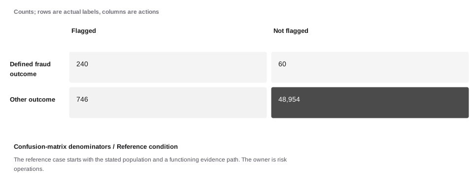
A concrete example. Precision, recall, and false-positive rate describe different conditional probabilities. The same threshold can create very different review demand when prevalence changes. The rule flags 986 of 50,000 labeled payments. Of those flags, 240 meet the synthetic target, giving 24.34% precision. It misses 60 target events. Under the stated cost assumptions, residual loss and operating friction total $23,574. The important result is the connection between the population, action, capacity, and outcome—not one isolated score.
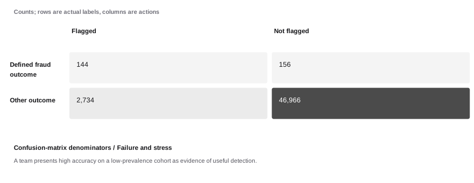
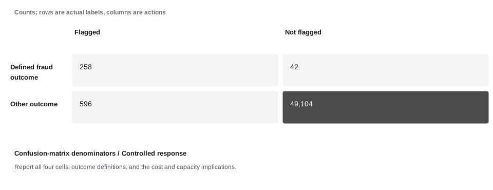
When the assumption fails. A team presents high accuracy on a low-prevalence cohort as evidence of useful detection. Report all four cells, outcome definitions, and the cost and capacity implications. The following worked sequence shows the reference condition, a stress condition, and a response condition with explicit synthetic data. These are comparative assumptions, not measured causal effects.
Precision, recall, and false-positive rate describe different conditional probabilities. The same threshold can create very different review demand when prevalence changes.
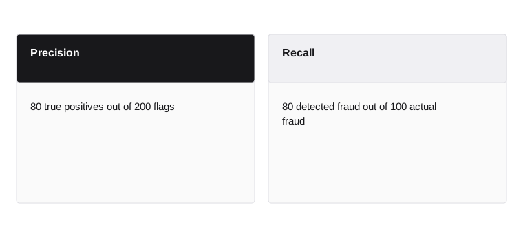
- Precision
- 80 true positives out of 200 flags
- Recall
- 80 detected fraud out of 100 actual fraud
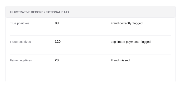
Confusion-matrix example
Illustrative data; not a real customer record or a prescribed policy.
- True positives80
Fraud correctly flagged
- False positives120
Legitimate payments flagged
- False negatives20
Fraud missed
One accuracy number can hide important errors
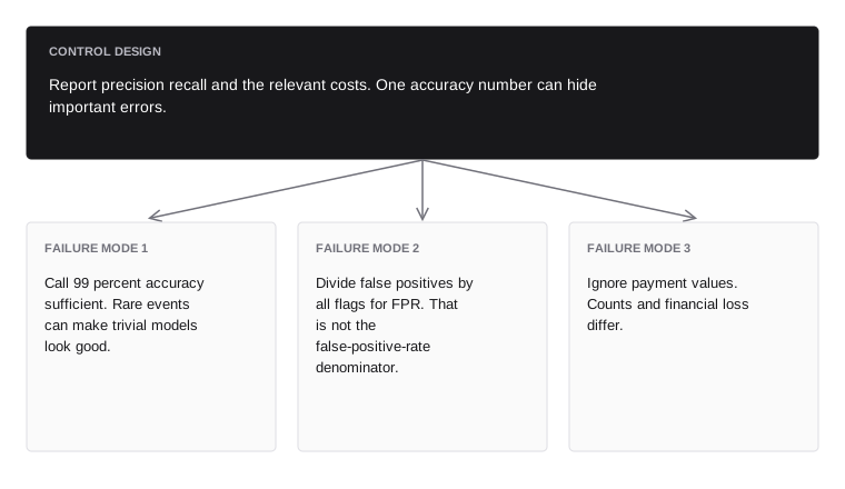
Report precision recall and the relevant costs. One accuracy number can hide important errors.
- Failure mode 1avoid
- Call 99 percent accuracy sufficient. Rare events can make trivial models look good.
- Failure mode 2avoid
- Divide false positives by all flags for FPR. That is not the false-positive-rate denominator.
- Failure mode 3avoid
- Ignore payment values. Counts and financial loss differ.
Calibrate probabilities before using dollars
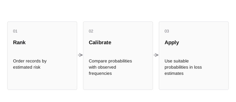
- RankOrder records by estimated risk
- CalibrateCompare probabilities with observed frequencies
- ApplyUse suitable probabilities in loss estimates
A calibrated probability estimate should correspond to observed outcome frequency in comparable groups, within sampling uncertainty. Ranking quality and calibration differ. A model can sort risky payments well while overstating their absolute probability.
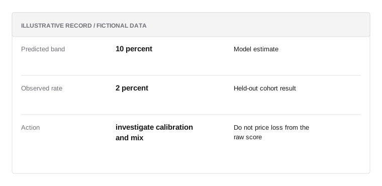
Use held-out data appropriate to the deployment population and examine reliability across score bands and segments. If payments assigned 10 percent risk develop about 2 percent observed fraud, the score may be miscalibrated or the evaluation population may differ. Expected-loss decisions need probability meaning, not just a useful ranking. Calibration itself can drift as behavior and selection change.
Calibration compares predicted probabilities with observed frequencies in an appropriate evaluation set. Among sufficiently many events predicted near 2%, the observed positive rate should be near 2% if the probabilities are well calibrated for that setting. This does not mean any particular event will produce 2% of a loss. It also does not guarantee calibration after the traffic or policy changes. A model can rank risky events well and still produce probabilities that are unsuitable for expected-dollar calculations without further work.
Inside the mechanism. A calibrated probability has a frequency interpretation for comparable predictions in the evaluated population. Ranking quality alone does not establish that interpretation. Reliability diagrams compare predicted probabilities with observed frequencies in bins, with uncertainty and sample size considered. Fit calibration using data separated from the model’s fitting data and evaluate on appropriate held-out observations. A lower Brier score can reflect discrimination as well as calibration, so it is not a pure calibration verdict.
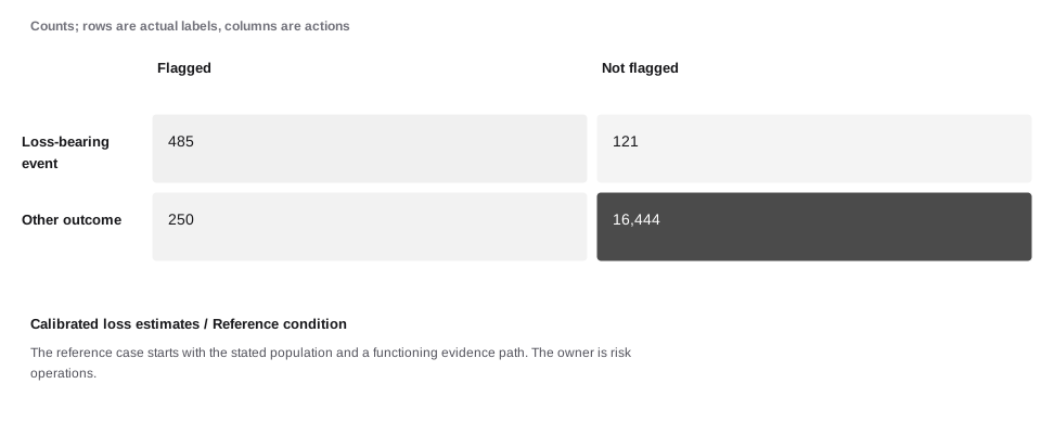
A concrete example. Ranking separates higher-risk cases from lower-risk cases. Calibration checks whether stated probabilities agree with observed outcome frequencies in comparable groups. The rule flags 735 of 17,300 mature decisions. Of those flags, 485 meet the synthetic target, giving 65.99% precision. It misses 121 target events. Under the stated cost assumptions, residual loss and operating friction total $50,170. The important result is the connection between the population, action, capacity, and outcome—not one isolated score.
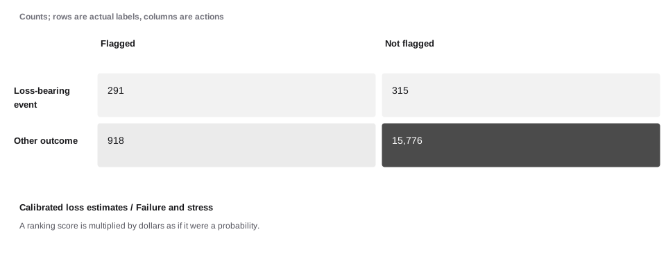
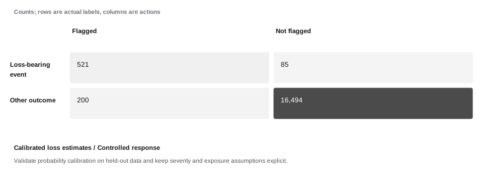
When the assumption fails. A ranking score is multiplied by dollars as if it were a probability. Validate probability calibration on held-out data and keep severity and exposure assumptions explicit. The following worked sequence shows the reference condition, a stress condition, and a response condition with explicit synthetic data. These are comparative assumptions, not measured causal effects.
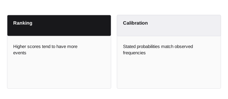
Ranking separates higher-risk cases from lower-risk cases. Calibration checks whether stated probabilities agree with observed outcome frequencies in comparable groups.
- Ranking
- Higher scores tend to have more events
- Calibration
- Stated probabilities match observed frequencies
Calibration check
Illustrative data; not a real customer record or a prescribed policy.
- Predicted band10 percent
Model estimate
- Observed rate2 percent
Held-out cohort result
- Actioninvestigate calibration and mix
Do not price loss from the raw score
A ranking score is not automatically a probability
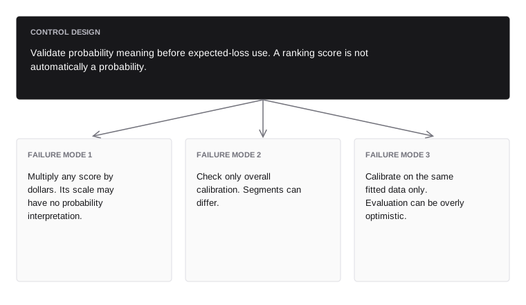
Validate probability meaning before expected-loss use. A ranking score is not automatically a probability.
- Failure mode 1avoid
- Multiply any score by dollars. Its scale may have no probability interpretation.
- Failure mode 2avoid
- Check only overall calibration. Segments can differ.
- Failure mode 3avoid
- Calibrate on the same fitted data only. Evaluation can be overly optimistic.
Split data by time and entity
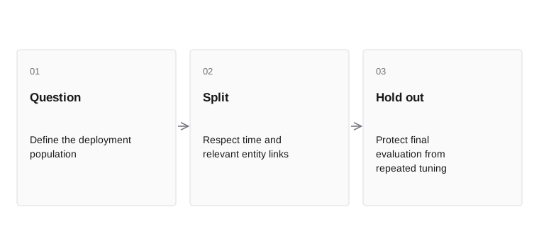
- QuestionDefine the deployment population
- SplitRespect time and relevant entity links
- Hold outProtect final evaluation from repeated tuning
Random splits can leak related records across training and evaluation. The same account, device cluster, or merchant can appear in both sets, making generalization look easier than it is. Temporal splits better reflect predicting later activity, but they also need entity and label-availability checks.
Define the evaluation question: future activity from known customers, new customers, new merchants, or another population. Choose splits that test it. Keep model selection separate from final evaluation. Repeatedly tuning against a holdout turns it into development data even if the filename still says test.
Inside the mechanism. Split data according to the leakage mechanism. Time separation prevents later observations from entering earlier evaluation; entity separation reduces reuse of related identities or coordinated groups across partitions. Both may be necessary. Preserve the feature availability cutoff and label maturity window. A random row split can look excellent while measuring memorization of shared entities or future information unavailable to production.
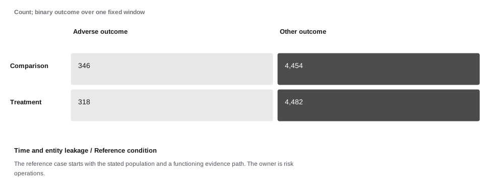
A concrete example. A random row split can put the same customer, device cluster, or future-derived feature on both sides of evaluation. Apparent performance can then reflect leakage. The comparison arm has 346/4800 adverse outcomes (7.21%) and the treatment arm has 318/4800 (6.62%). The absolute difference is -0.58 percentage points, with an illustrative large-sample 95% interval from -1.60 to 0.43. Interpretation depends on assignment integrity, outcome maturity, independence, and the actual decision being evaluated.
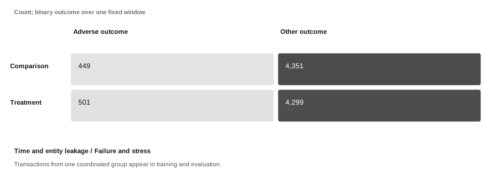
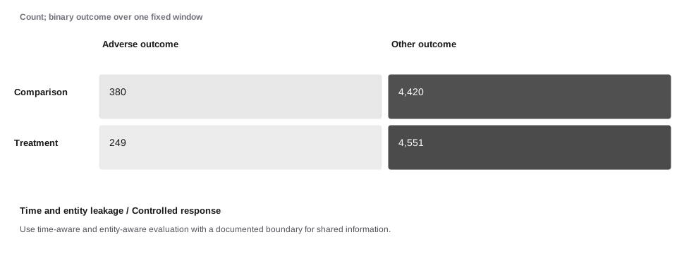
When the assumption fails. Transactions from one coordinated group appear in training and evaluation. Use time-aware and entity-aware evaluation with a documented boundary for shared information. The following worked sequence shows the reference condition, a stress condition, and a response condition with explicit synthetic data. These are comparative assumptions, not measured causal effects.
A random row split can put the same customer, device cluster, or future-derived feature on both sides of evaluation. Apparent performance can then reflect leakage.
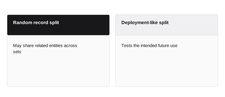
- Random record split
- May share related entities across sets
- Deployment-like split
- Tests the intended future use
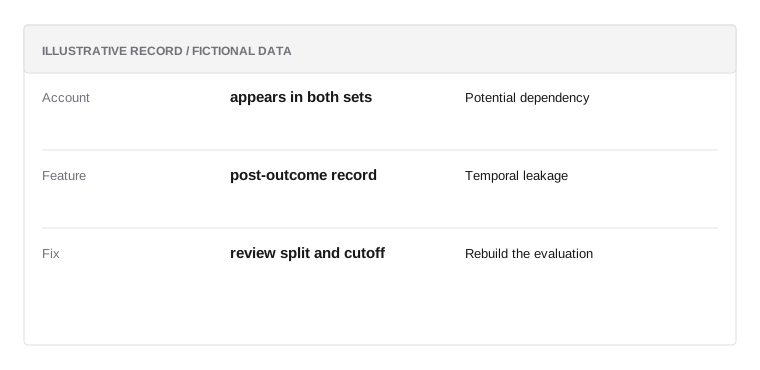
Split audit
Illustrative data; not a real customer record or a prescribed policy.
- Accountappears in both sets
Potential dependency
- Featurepost-outcome record
Temporal leakage
- Fixreview split and cutoff
Rebuild the evaluation
Record randomness alone is not enough
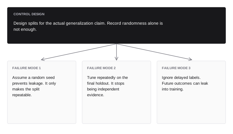
Design splits for the actual generalization claim. Record randomness alone is not enough.
- Failure mode 1avoid
- Assume a random seed prevents leakage. It only makes the split repeatable.
- Failure mode 2avoid
- Tune repeatedly on the final holdout. It stops being independent evidence.
- Failure mode 3avoid
- Ignore delayed labels. Future outcomes can leak into training.
Monitor the model as part of a system
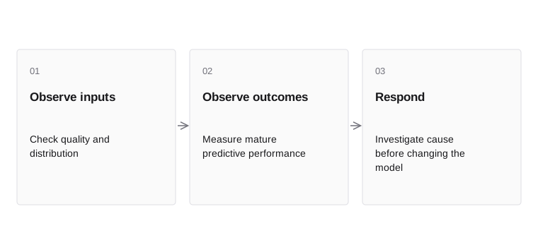
- Observe inputsCheck quality and distribution
- Observe outcomesMeasure mature predictive performance
- RespondInvestigate cause before changing the model
Track input quality, score distribution, calibration, ranking, latency, coverage, and mature outcomes. Data drift means inputs changed; performance drift means outcome quality changed. One can occur without the other.
Define action thresholds with owners and context. A score-distribution shift may come from a new merchant mix rather than a model defect. A stable score distribution can still hide deteriorating calibration. Monitor the decision policy and human overrides too. Customers experience the complete system, not an isolated model artifact.
Inside the mechanism. Monitor the decision system around the model: input quality, score distribution, action delivery, queue capacity, overrides, mature outcomes, and relevant population changes. A stable score distribution does not prove stable performance. Labels can stop arriving while scores remain normal. Tie alerts to a supported response and distinguish data faults, population drift, and model degradation before choosing a remedy.
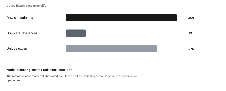
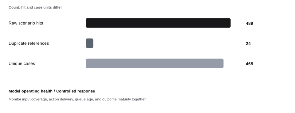
A concrete example. A model can retain its score distribution while its inputs, labels, or downstream actions fail. Monitoring should join technical quality with mature business outcomes. The daily source population is 39,000 items, but 780 are outside the completed monitoring run. The included population creates 459 hits and 376 unique cases. With 95 cases already open and capacity for 460, the queue closes at 11. Coverage, duplicate work, and staffing are separate causes; reducing one number does not prove that the overall control improved.
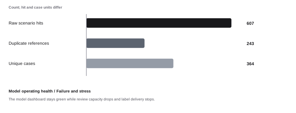
When the assumption fails. The model dashboard stays green while review capacity drops and label delivery stops. Monitor input coverage, action delivery, queue age, and outcome maturity together. The following worked sequence shows the reference condition, a stress condition, and a response condition with explicit synthetic data. These are comparative assumptions, not measured causal effects.
A model can retain its score distribution while its inputs, labels, or downstream actions fail. Monitoring should join technical quality with mature business outcomes.
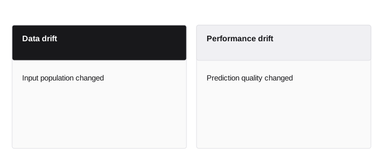
- Data drift
- Input population changed
- Performance drift
- Prediction quality changed
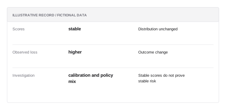
Monitoring example
Illustrative data; not a real customer record or a prescribed policy.
- Scoresstable
Distribution unchanged
- Observed losshigher
Outcome change
- Investigationcalibration and policy mix
Stable scores do not prove stable risk
The model is one part of the customer decision
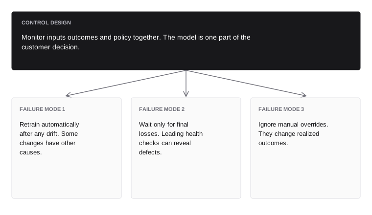
Monitor inputs outcomes and policy together. The model is one part of the customer decision.
- Failure mode 1avoid
- Retrain automatically after any drift. Some changes have other causes.
- Failure mode 2avoid
- Wait only for final losses. Leading health checks can reveal defects.
- Failure mode 3avoid
- Ignore manual overrides. They change realized outcomes.
Chapter connections
This chapter builds on Decision engines, rules, and reliable execution. Continue with Experiments, causal effects, and risk tradeoffs to follow the next part of the system. Use the glossary for terminology and risk mathematics for formulas and worked calculations.