
Calibrated loss estimates
Calibrate probabilities before using dollars
The evaluated population
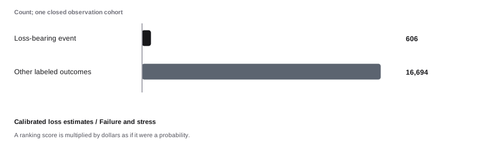
The cohort contains 17,300 mature decisions, of which 606 have the defined synthetic outcome: Loss-bearing event. The outcome is known by construction here. In production, label uncertainty and selection must be recorded separately.
Figure data and text version
| Outcome | Count |
|---|---|
| Loss-bearing event | 606 |
| Other labeled outcomes | 16,694 |
Ranking separates higher-risk cases from lower-risk cases. Calibration checks whether stated probabilities agree with observed outcome frequencies in comparable groups.
A ranking score is multiplied by dollars as if it were a probability.
All amounts, rates, capacity limits, and outcomes in this case are synthetic. The three conditions are separate assumptions for comparison. A better result in the response condition is not measured proof that the proposed control causes that improvement. The figures expose the calculation and its limits; a real deployment needs its own evidence.
Read the result
The rule flags 1,209 of 17,300 mature decisions. Of those flags, 291 meet the synthetic target, giving 24.07% precision. It misses 315 target events. Under the stated cost assumptions, residual loss and operating friction total $129,126. The important result is the connection between the population, action, capacity, and outcome—not one isolated score.
Model inputs and calculated values
Inputs below are the case-specific values. Each figure states the condition-specific assumptions and units used in its calculation. Calculated values are rounded for display.
| Input | Value |
|---|---|
| population | 17,300 |
| prevalence | 0.035 |
| severity | 380 |
| Calculated value | Result |
|---|---|
| population | 17,300 |
| positive | 606 |
| negative | 16,694 |
| tp | 291 |
| fp | 918 |
| fn | 315 |
| tn | 15,776 |
| loss | 119,700 |
| severity | 380 |
| precision | 24.07 |
| recall | 48.02 |
Four outcomes of the rule
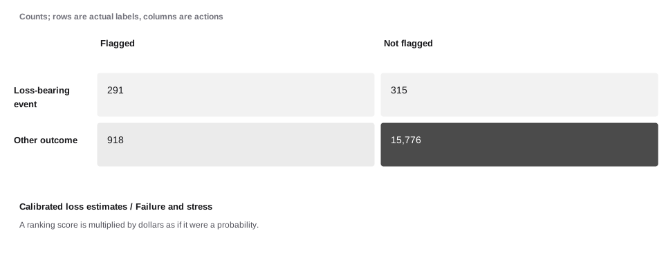
The rule flags 291 synthetic positives and 918 negatives. It misses 315 positives. A flagged item is a decision to intervene; it is not proof of fraud, a legal prohibition, or any other real-world conclusion.
Figure data and text version
| Known outcome | Flagged | Not flagged |
|---|---|---|
| Loss-bearing event | 291 | 315 |
| Other outcome | 918 | 15,776 |
Three rates with different denominators
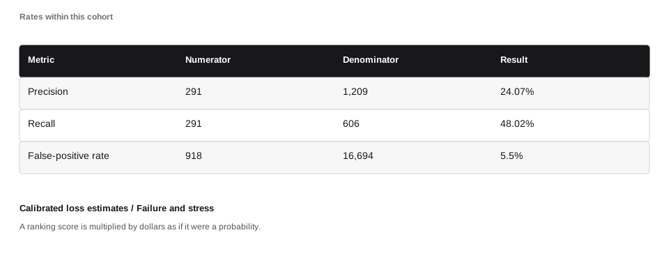
Precision is 24.07%, recall is 48.02%, and the false-positive rate is 5.5%. Changing the denominator changes the meaning. This record keeps each numerator attached to the population from which it came.
Figure data and text version
| Metric | Numerator | Denominator | Result |
|---|---|---|---|
| Precision | 291 | 1,209 | 24.07% |
| Recall | 291 | 606 | 48.02% |
| False-positive rate | 918 | 16,694 | 5.5% |
Precision changes with prevalence
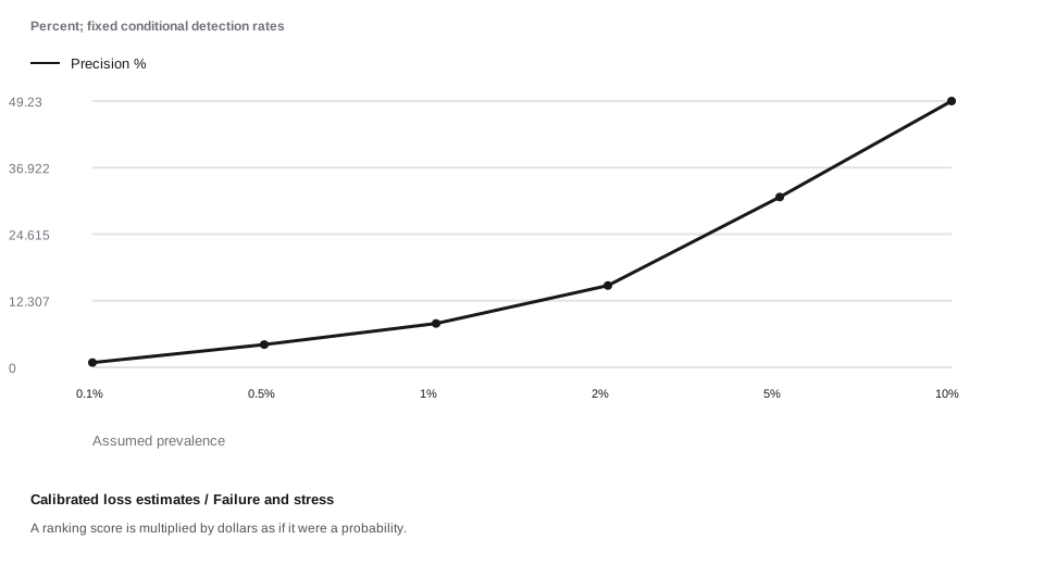
This sensitivity plot holds recall at 48% and false-positive rate at 5.5%, then changes prevalence. It is an algebraic comparison, not a forecast. Even unchanged detection quality can produce a very different review queue when the base rate changes. Horizontal positions are the labeled observations or scenarios; equal spacing does not imply equal numerical increments.
Figure data and text version
| Assumed prevalence | Precision % |
|---|---|
| 0.1% | 0.87 |
| 0.5% | 4.2 |
| 1% | 8.1 |
| 2% | 15.12 |
| 5% | 31.48 |
| 10% | 49.23 |
The threshold trade-off
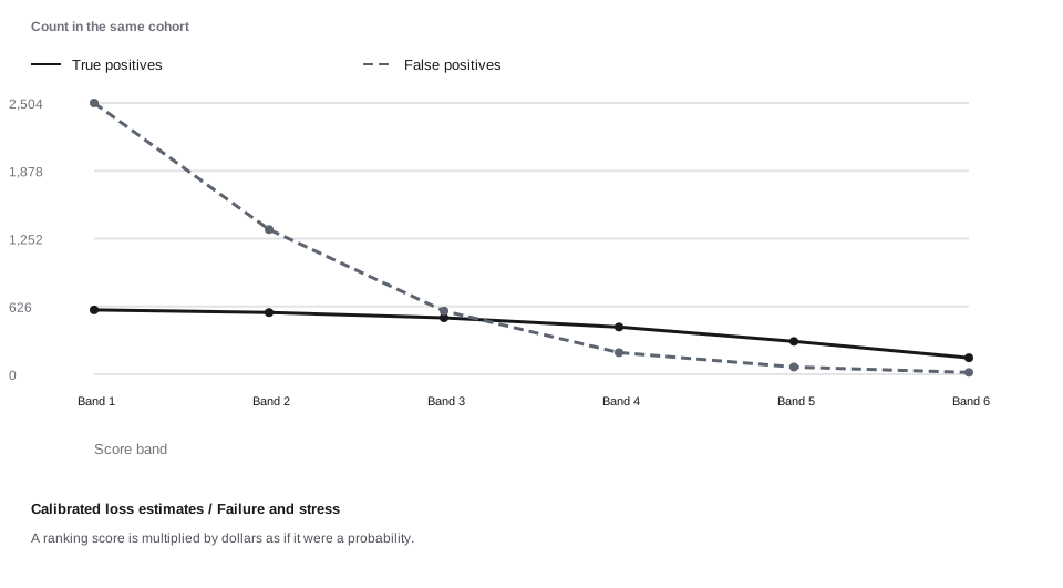
Six illustrative score bands use a stated pair of detection rates. Lower sensitivity can reduce false alarms but miss more target events. These points do not come from a trained model and do not establish the best operating threshold. Horizontal positions are the labeled observations or scenarios; equal spacing does not imply equal numerical increments.
Figure data and text version
| Score band | True positives | False positives |
|---|---|---|
| Band 1 | 594 | 2,504 |
| Band 2 | 570 | 1,336 |
| Band 3 | 521 | 584 |
| Band 4 | 436 | 200 |
| Band 5 | 303 | 67 |
| Band 6 | 152 | 17 |
A transparent loss-and-friction calculation
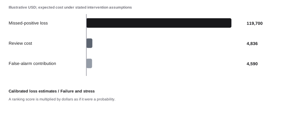
At $380 severity per missed synthetic positive, residual loss is $119,700. Review costs $4,836; lost contribution on false alarms is $4,590. The calculation assumes intervention prevents all flagged-positive loss and each false alarm loses the stated contribution. Relax those assumptions before applying it to a real policy.
Figure data and text version
| Cost component | USD |
|---|---|
| Missed-positive loss | 119,700 |
| Review cost | 4,836 |
| False-alarm contribution | 4,590 |
Observed outcomes mature over time
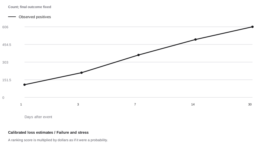
The final synthetic positive count is 606. Earlier observations reveal only a stated fraction. Comparing a day-1 cohort with a day-30 cohort would confuse label age with control quality. This curve models observation delay only; it does not change the final outcome. Horizontal positions are the labeled observations or scenarios; equal spacing does not imply equal numerical increments.
Figure data and text version
| Days after event | Observed positives |
|---|---|
| 1 | 109 |
| 3 | 212 |
| 7 | 364 |
| 14 | 497 |
| 30 | 606 |
Review demand and available capacity
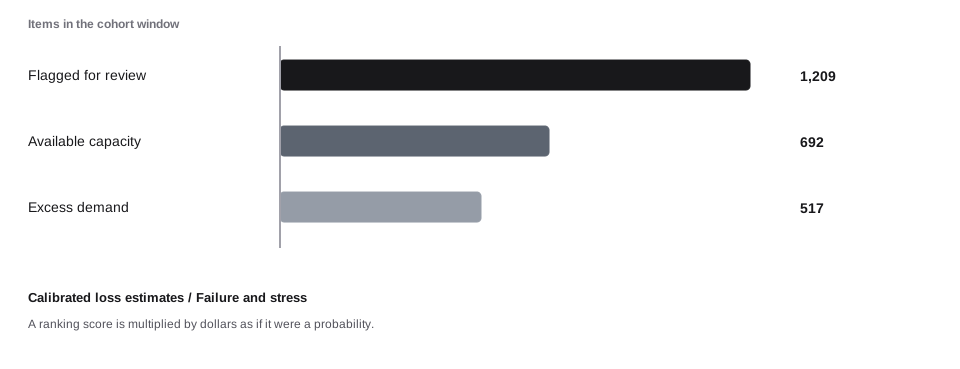
The flag count is 1,209. The comparison capacity is an illustrative 692 reviews per cohort window. A mathematical rule can be coherent while its resulting workload exceeds the operating team’s capacity. Capacity is not permission to ignore an applicable mandatory control.
Figure data and text version
| Queue measure | Items |
|---|---|
| Flagged for review | 1,209 |
| Available capacity | 692 |
| Excess demand | 517 |
A feature is an observation with provenance
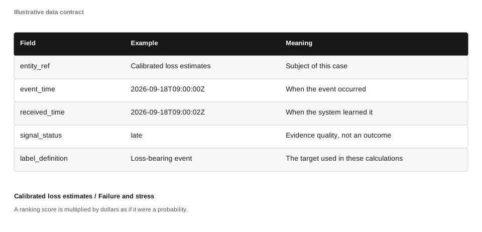
This evidence contract supports calibrate probabilities before using dollars. A value needs its event time, arrival time, scope, and source. Keeping unavailable evidence distinct from a measured zero prevents an outage from becoming a falsely reassuring feature.
Figure data and text version
| Field | Example | Meaning |
|---|---|---|
| entity_ref | Calibrated loss estimates | Subject of this case |
| event_time | 2026-09-18T09:00:00Z | When the event occurred |
| received_time | 2026-09-18T09:00:02Z | When the system learned it |
| signal_status | late | Evidence quality, not an outcome |
| label_definition | Loss-bearing event | The target used in these calculations |
Missing evidence changes the observed population
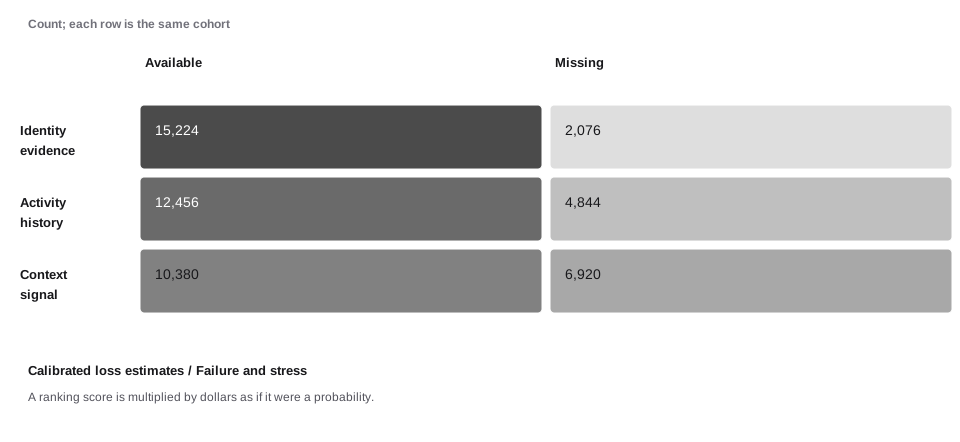
The cells show an explicitly constructed completeness profile for three signal groups. The stress condition removes more history and device evidence. Missingness does not prove the target outcome; it changes what the decision process knows.
Figure data and text version
| Signal group | Available | Missing |
|---|---|---|
| Identity evidence | 15,224 | 2,076 |
| Activity history | 12,456 | 4,844 |
| Context signal | 10,380 | 6,920 |
Evidence, score, and action remain separate
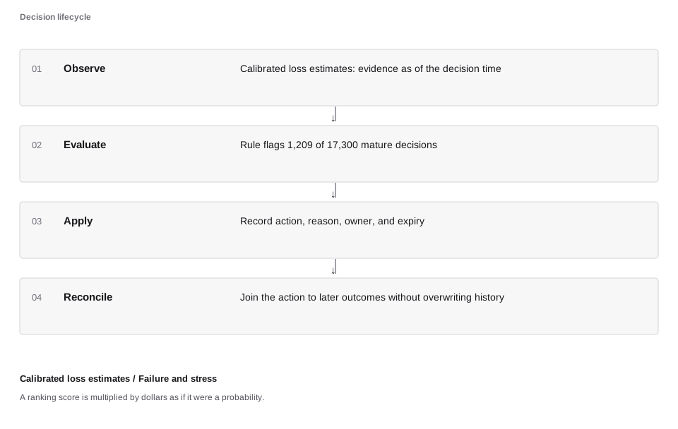
The policy can use calibrate probabilities before using dollars only within its approved scope. The action record must retain which evidence was available, which model or rule ran, and which action was actually applied. The final action can differ from the score recommendation when a separate constraint applies.
Figure data and text version
| Stage | Record |
|---|---|
| Observe | Calibrated loss estimates: evidence as of the decision time |
| Evaluate | Rule flags 1,209 of 17,300 mature decisions |
| Apply | Record action, reason, owner, and expiry |
| Reconcile | Join the action to later outcomes without overwriting history |
What the result cannot establish
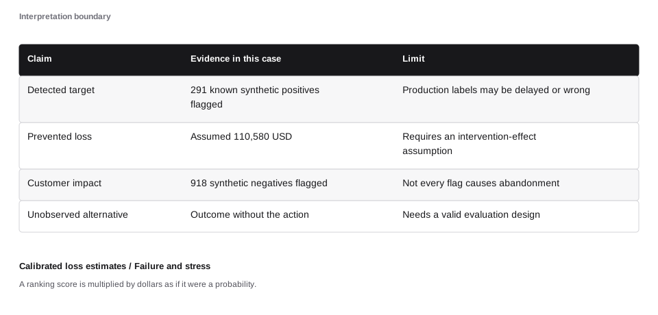
Observed classifications do not reveal every counterfactual. The synthetic labels make arithmetic possible, but production decline data is selected by prior policy. Keep measured outcomes, assumed prevention, and unknown alternatives separate when reporting impact.
Figure data and text version
| Claim | Evidence in this case | Limit |
|---|---|---|
| Detected target | 291 known synthetic positives flagged | Production labels may be delayed or wrong |
| Prevented loss | Assumed 110,580 USD | Requires an intervention-effect assumption |
| Customer impact | 918 synthetic negatives flagged | Not every flag causes abandonment |
| Unobserved alternative | Outcome without the action | Needs a valid evaluation design |
Connect the result to the system
Validate probability calibration on held-out data and keep severity and exposure assumptions explicit.
Check the population, evidence, permitted action, and actual effect together. A balanced calculation can still use the wrong population; a successful response can still leave an unknown financial outcome. The case’s numerical result applies only to its stated assumptions.
Sources and further reading
The chapter sources support the concepts and scope. They do not prescribe the synthetic model rates.