
Rule release evidence
Release rules with rollback evidence
Start with the assigned population
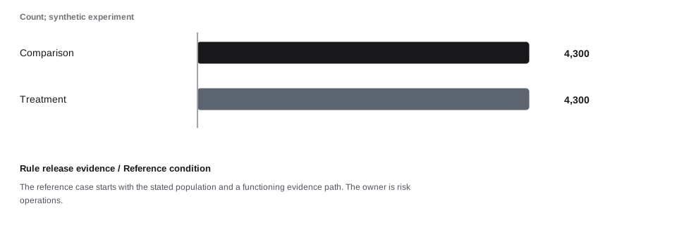
This teaching experiment assigns 4,300 eligible units to comparison and 4,300 to treatment. The units are eligible accounts. Mandatory controls are outside the experimental choice. Eligibility and assignment are defined before observing outcomes.
Figure data and text version
| Assigned arm | Units |
|---|---|
| Comparison | 4,300 |
| Treatment | 4,300 |
A release can change approvals, losses, queue demand, and customer friction at once. A rollback also needs to address decisions already made under the changed policy.
The reference case starts with the stated population and a functioning evidence path. The owner is risk operations.
All amounts, rates, capacity limits, and outcomes in this case are synthetic. The three conditions are separate assumptions for comparison. A better result in the response condition is not measured proof that the proposed control causes that improvement. The figures expose the calculation and its limits; a real deployment needs its own evidence.
Read the result
The comparison arm has 194/4300 adverse outcomes (4.51%) and the treatment arm has 178/4300 (4.14%). The absolute difference is -0.37 percentage points, with an illustrative large-sample 95% interval from -1.23 to 0.49. Interpretation depends on assignment integrity, outcome maturity, independence, and the actual decision being evaluated.
Model inputs and calculated values
Inputs below are the case-specific values. Each figure states the condition-specific assumptions and units used in its calculation. Calculated values are rounded for display.
| Input | Value |
|---|---|
| population | 8,600 |
| clusterSize | 6 |
| correlation | 0.04 |
| rate | 0.045 |
| Calculated value | Result |
|---|---|
| n | 8,600 |
| nc | 4,300 |
| nt | 4,300 |
| yc | 194 |
| yt | 178 |
| effect | -0.0037 |
| lower | -0.0123 |
| upper | 0.0049 |
| clusterSize | 6 |
| icc | 0.016 |
| effectiveN | 7,962.963 |
Retain events and nonevents in both arms
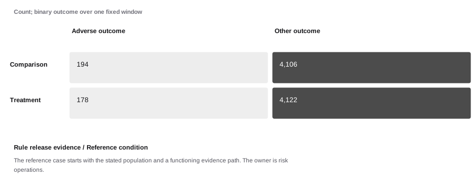
The defined adverse outcome occurs 194 times in comparison and 178 times in treatment. Each row includes every assigned unit under this complete-outcome illustration. Omitting nonevents or unresolved cases changes the denominator and the estimand.
Figure data and text version
| Assigned arm | Adverse outcome | Other outcome |
|---|---|---|
| Comparison | 194 | 4,106 |
| Treatment | 178 | 4,122 |
Absolute and relative effects answer different questions
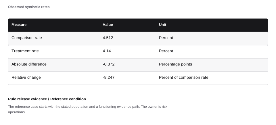
Treatment minus comparison is -0.37 percentage points. The relative change is -8.25% when the comparison rate is nonzero. A percentage-point difference and a percentage change must not share the same label.
Figure data and text version
| Measure | Value | Unit |
|---|---|---|
| Comparison rate | 4.512 | Percent |
| Treatment rate | 4.14 | Percent |
| Absolute difference | -0.372 | Percentage points |
| Relative change | -8.247 | Percent of comparison rate |
Each arm’s rate has sampling uncertainty
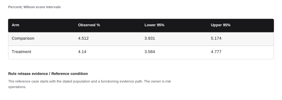
The 95% Wilson intervals are [3.93, 5.17]% and [3.58, 4.78]%. These intervals use independent Bernoulli sampling assumptions. Shared customers or merchants can violate that independence and require an appropriate clustered analysis.
Figure data and text version
| Arm | Observed % | Lower 95% | Upper 95% |
|---|---|---|---|
| Comparison | 4.512 | 3.931 | 5.174 |
| Treatment | 4.14 | 3.584 | 4.777 |
Uncertainty in the difference
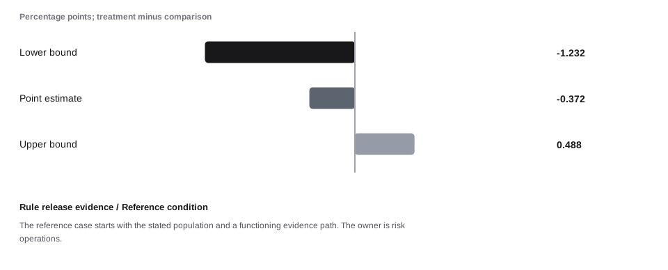
The normal-approximation 95% interval for treatment minus comparison is [-1.23, 0.49] percentage points. It is a teaching large-sample interval, not a replacement for the analysis appropriate to the design, low counts, sequential monitoring, or multiple comparisons.
Figure data and text version
| Difference measure | Percentage points |
|---|---|
| Lower bound | -1.232 |
| Point estimate | -0.372 |
| Upper bound | 0.488 |
A fixed outcome horizon prevents premature comparison
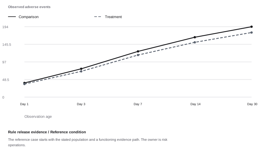
Both arms use the same explicitly constructed maturation fractions. Earlier data can undercount the final outcome even when assignment is correct. Stopping at the first favorable partial result also changes the statistical interpretation unless the monitoring design accounts for it. Horizontal positions are the labeled observations or scenarios; equal spacing does not imply equal numerical increments.
Figure data and text version
| Observation age | Comparison events | Treatment events |
|---|---|---|
| Day 1 | 39 | 36 |
| Day 3 | 78 | 71 |
| Day 7 | 126 | 116 |
| Day 14 | 165 | 151 |
| Day 30 | 194 | 178 |
Assignment and received treatment differ
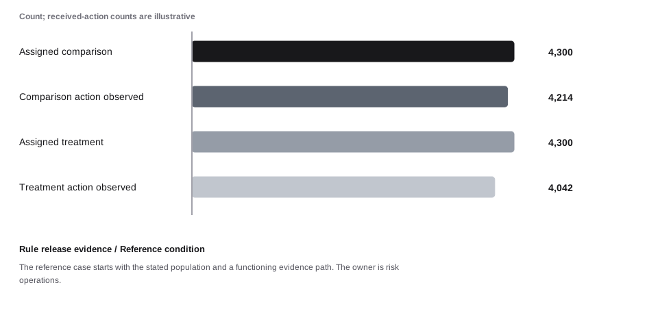
4300 units are assigned to treatment, while 4042 receive the modeled action. The primary assignment-based comparison retains all assigned units. Restricting to action recipients selects a post-assignment subgroup and can introduce bias.
Figure data and text version
| Population | Units |
|---|---|
| Assigned comparison | 4,300 |
| Comparison action observed | 4,214 |
| Assigned treatment | 4,300 |
| Treatment action observed | 4,042 |
Correlated units reduce independent information
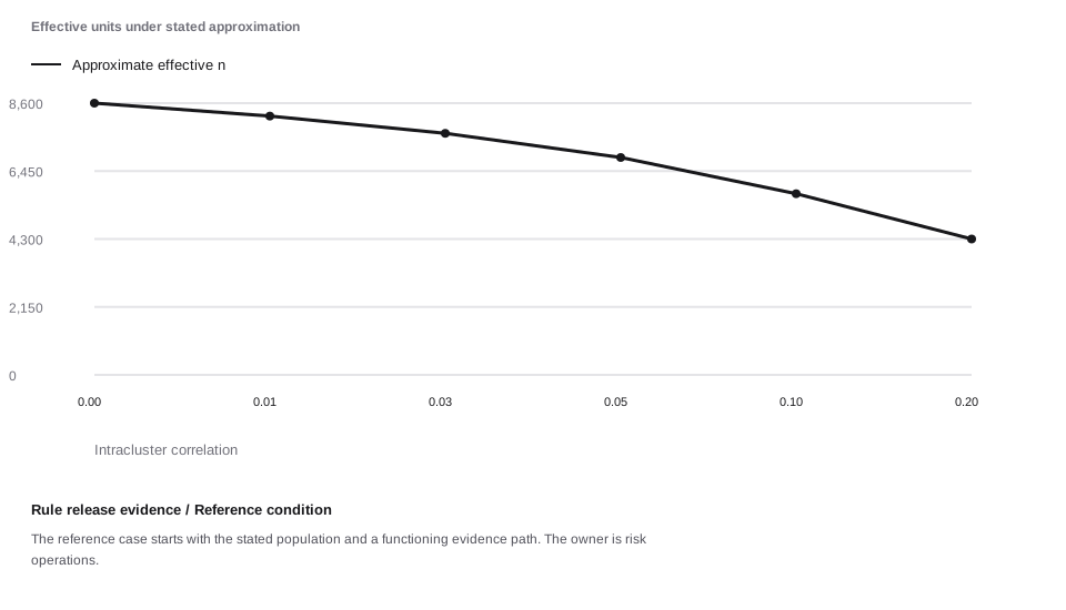
The design-effect illustration is 1 + (m − 1)ρ with cluster size m = 6. At the case’s assumed ρ = 0.016, the design effect is 1.080 and n/design-effect is about 7,963.0. This approximation assumes a simple equal-cluster design; it is not a universal effective-sample-size formula. Horizontal positions are the labeled observations or scenarios; equal spacing does not imply equal numerical increments.
Figure data and text version
| Intracluster correlation | Approximate effective n |
|---|---|
| 0.00 | 8,600 |
| 0.01 | 8,190.5 |
| 0.03 | 7,644.4 |
| 0.05 | 6,880 |
| 0.10 | 5,733.3 |
| 0.20 | 4,300 |
Segment totals must reconcile to the whole
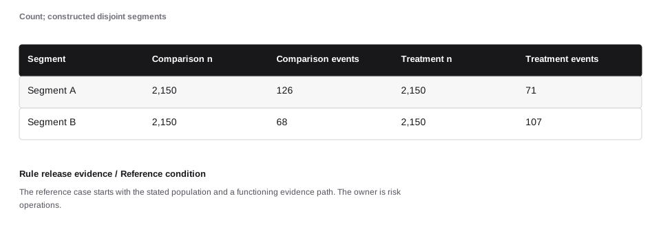
The two synthetic segments partition each arm. Their outcome counts add back to the original totals. Segment effects can differ from the overall effect, but small cells, selection, and multiple comparisons must be considered before interpreting a subgroup result.
Figure data and text version
| Segment | Comparison n | Comparison events | Treatment n | Treatment events |
|---|---|---|---|---|
| Segment A | 2,150 | 126 | 2,150 | 71 |
| Segment B | 2,150 | 68 | 2,150 | 107 |
The primary outcome is only one decision input
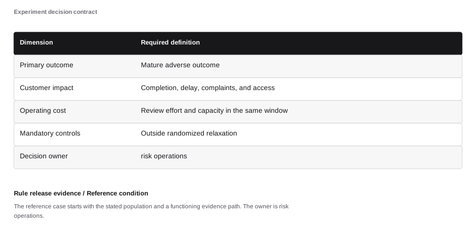
The primary target is Mature adverse outcome. A release also considers customer friction, queue capacity, required controls, and the uncertainty of the result. A favorable loss metric cannot justify an action that violates a separate obligation.
Figure data and text version
| Dimension | Required definition |
|---|---|
| Primary outcome | Mature adverse outcome |
| Customer impact | Completion, delay, complaints, and access |
| Operating cost | Review effort and capacity in the same window |
| Mandatory controls | Outside randomized relaxation |
| Decision owner | risk operations |
Specify the analysis before observing the result
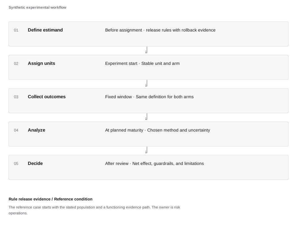
The protocol fixes assignment, exclusions, metrics, outcome maturity, and the comparison method. Changing these after seeing results can make an ordinary noise fluctuation look like an improvement. Amendments need a documented reason and a clear distinction between confirmatory and exploratory work.
Figure data and text version
| Stage | Timing | Record |
|---|---|---|
| Define estimand | Before assignment | release rules with rollback evidence |
| Assign units | Experiment start | Stable unit and arm |
| Collect outcomes | Fixed window | Same definition for both arms |
| Analyze | At planned maturity | Chosen method and uncertainty |
| Decide | After review | Net effect, guardrails, and limitations |
What this example establishes and omits
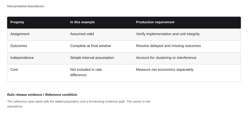
The arithmetic shows how the stated counts become rates, differences, and intervals. It does not prove a causal effect in production. Causal interpretation requires a valid assignment process, appropriate handling of interference and missing outcomes, and analysis consistent with the design.
Figure data and text version
| Property | In this example | Production requirement |
|---|---|---|
| Assignment | Assumed valid | Verify implementation and unit integrity |
| Outcomes | Complete at final window | Resolve delayed and missing outcomes |
| Independence | Simple interval assumption | Account for clustering or interference |
| Cost | Not included in rate difference | Measure net economics separately |
Connect the result to the system
Predefine outcome windows, operational limits, and a reversible release path.
Check the population, evidence, permitted action, and actual effect together. A balanced calculation can still use the wrong population; a successful response can still leave an unknown financial outcome. The case’s numerical result applies only to its stated assumptions.
Sources and further reading
The chapter sources support the concepts and scope. They do not prescribe the synthetic model rates.